
Modelling the effects of Spartina alterniflora invasion on the landscape succession of Yancheng coastal natural wetlands, China
- Published
- Accepted
- Received
- Academic Editor
- Stuart Pimm
- Subject Areas
- Biogeography, Ecology, Ecosystem Science, Plant Science, Spatial and Geographic Information Science
- Keywords
- Yancheng, Native coastal wetlands, Invasive alien species, Spartina alterniflora, Cellular-automaton Markov model, Spatial and temporal changes, Sustainable development
- Copyright
- © 2020 Dai et al.
- Licence
- This is an open access article distributed under the terms of the Creative Commons Attribution License, which permits unrestricted use, distribution, reproduction and adaptation in any medium and for any purpose provided that it is properly attributed. For attribution, the original author(s), title, publication source (PeerJ) and either DOI or URL of the article must be cited.
- Cite this article
- 2020. Modelling the effects of Spartina alterniflora invasion on the landscape succession of Yancheng coastal natural wetlands, China. PeerJ 8:e10400 https://doi.org/10.7717/peerj.10400
Abstract
Background
The Yancheng coastal natural wetlands (YCNR) are well-preserved silty tidal flat wetlands in China. Due to the severe invasion of Spartina alterniflora, the native ecosystem has undergone great changes. The successful invasion of S. alterniflora reduced the biodiversity of the YCNR, changed the structure and function of the local ecosystem, and eventually led to the degradation of the ecosystem and the loss of ecosystem function and service. Fully understanding the impact of an alien species invasion on YCNR succession is an important prerequisite for protecting and restoring the wetlands.
Methods
In this study, remote sensing, GIS technology, and a cellular-automaton Markov model were used to simulate the natural succession process of native ecosystems without being affected by alien species. By comparing the landscape of the YCNR with the model simulation results, we gained a better understanding of how alien species affect native landscape-scale ecosystems.
Results
During the natural succession of the coastal native wetland ecosystem in the YCNR, the pioneer species S. alterniflora occupied the mudflats and expanded seaward. The whole area expanded and moved seaward with an average annual movement of 58.23 m. Phragmites australis seemed to dominate the competition with S. salsa communities, and the area gradually expanded with an average annual movement of 39.89 m. The invasion of S. alterniflora changed the native ecosystem’s spatial succession process, causing the S. salsa ecosystem to be stressed by ecosystems on the side of the sea (S. alterniflora) and that of land (P. australis). The area of the seaward-expanding P. australis ecosystem has been declining. Under a reasonable protected area policy, human activities have enhanced the succession rate of the P. australis ecosystem and have had a small impact on the ecological spatial succession of S. salsa and S. alterniflora.
Introduction
Coastal wetlands are located in the land-sea transition zone (Gómez, White & Wulder, 2016), which is a marginal area and one of the most valuable ecosystems on Earth’s surface (Barbier et al., 2011; Lotze et al., 2006; Smith, 2003). Coastal wetlands have unique functions that cannot be replaced. They are the most biodiverse and highly productive ecosystems (Barbier et al., 2011). They are also the most sensitive areas of the atmosphere, hydrosphere, pedosphere, and biosphere energy and material exchange (Chmura et al., 2003; Jiang et al., 2015; Lotze et al., 2006). Spartina alterniflora was introduced to the Yancheng coastal intertidal zone in 1979 (Xu et al., 1989), and a continuous area of S. alterniflora has formed since 2000. By 2017, the width of S. alterniflora was 1.88 km, the length was 12.90 km and the area was 3,925 ha. The Yancheng coastal natural wetlands (YCNR) are a wetland type that grows and develops in the muddy intertidal zone. Affected by ocean tides, the natural wetland landscape is mainly composed of Phragmites australis marshes, Suaeda salsa marshes, and mudflats; it develops from land seaward, and it is parallel to the coast (Ou et al., 2004; Zhou et al., 2009). S. alterniflora is the main invasive species in China’s coastal zone, and Yancheng is the most significant area affected by S. alterniflora invasion. Invasive species directly or indirectly reduce the biodiversity of an invaded area. The consequences are changes in the structure and function of the ecosystem and eventually the degradation of the native ecosystem, reducing its ecological function. Evidence has shown that S. alterniflora invasion can have serious ecological consequences by changing the terrain of the intertidal zone (Daehler & Strong, 1996; Gleason et al., 1979), hindering the flow of tidal ditches and water channels, replacing indigenous plants (Callaway & Josselyn, 1992; Chen et al., 2004), crossing with indigenous plants of the same genus, causing the loss of indigenous-plant genotypes or producing hybrids that are more invasive than their parents (Anttila et al., 1998; Ayres et al., 1999), reducing the density and species richness of large benthic invertebrates (Da Cunha Lana & Guiss, 1991; Luiting et al., 1997), hindering fish resource use (Cordell et al., 1998), and reducing key habitats for wintering and water-bird reproduction. Invasive S. alterniflora species not only cause biodiversity changes and ecosystem imbalances but also have an important impact on natural-wetland landscape succession. How to effectively manage and control invasive species is an issue of concern to governments and scientists around the world.
Spartina alterniflora, a perennial salt-tolerant plant, originated from the west coast of the Atlantic and the Gulf of Mexico, and it is the dominant plant in the low salt marsh of the coastal zone (Bortolus et al., 2019; Bortolus, Carlton & Schwindt, 2015; Peterson et al., 2014). S. alterniflora plays an important ecological role in the country of origin. It was unintentionally or intentionally introduced to many countries and regions around the world. It has been shown that there are a series of mechanisms that are beneficial to the survival and diffusion of S. alterniflora, for example, seeds, rhizomes, and asexual segments used for rapid propagation and diffusion (Daehler & Strong, 1994); additionally, the species is tolerant to a wide range of changes in ecological factors (Landin, 1991) and has ventilating tissue in the body that can utilize nutrients in the soil under low-oxygen conditions and strong interspecific competition ability (Bertness, 1991; Callaway & Josselyn, 1992; Daehler & Strong, 1996). S. alterniflora has become one of the most successful invasive plants in the global coastal salt marsh ecosystem and has received extensive attention. Since the introduction of S. alterniflora in the 1970s, it has rapidly expanded in coastal zones (Wang et al., 2018), and the stripe pattern of S. alterniflora, S. salsa, and P. australis, in turn, have expanded from the sea to the land (Sun et al., 2009; Yao et al., 2009).
The Aichi biodiversity target 9 and Sustainable Development Goal 15 targets clearly state that to better protect the diversity of local native ecosystems, we need to address problems such as S. alterniflora invasion and develop measures to manage species to prevent invasive alien species from exacerbating ecological damage. Current related research reveals the harmful effects of S. alterniflora invasion on regional ecological balance and marine economic development from the perspectives of the ecosystem, ecological processes, structures, and functionality (Chung, 2006; Lu & Zhang, 2013; Zhang, Jiang & Wang, 2009). However, research on how S. alterniflora invasion affects native-vegetation-landscape succession requires more attention. To reveal the influence of S. alterniflora on the landscape succession of native wetland ecosystems, eight remote-sensing imageries were used as the data source, and the cellular-automaton (CA) Markov model was used to solve two scientific problems on the landscape scale. First, how would the natural landscape of the YCNR develop without Spartina invasion? Second, how does S. alterniflora structurally affect local landscape succession?
These two scientific issues have important practical guidance for a deep understanding of the impact of S. alterniflora invasion on the natural wetland landscape in the intertidal zone of Yancheng, reasonable control of S. alterniflora, and protection of the native natural landscape system.
Materials & Methods
Study area
An intertidal zone that is typical of the S. alterniflora invasion in Yancheng was selected as the sample area (Fig. 1). This area is the core area of the Yancheng National Rare Birds Nature Reserve in Jiangsu, located at 119°53′45″∼121°18′12″E, 32°48′47″∼34°29′28″N. The reserve mainly protects rare wild animals, such as red-crowned cranes, and their habitat. The reserve is a member of the World Biosphere Reserve Network, a member of the Northeast Asian Crane Protection Network, and a member of the East Asian-Australasian Flyway Partnership. This wetland is one of the important wetlands in the Ramsar Convention and was listed as a World Natural Heritage Site in 2019. The sample area is bounded by the Xinyanggang River to the north and the Doulonggang River to the south. The east is bounded by a 6-m seawater isobath, and the west is bounded by the Sheyang Seawall Road, with an area of 23,830 hectares. The region is in the transition zone of the warm temperate and northern subtropical zones. It is mainly affected by a monsoon climate. The annual average temperature is 13.7–14.6 °C, the annual extreme minimum temperature is −10 °C (January), and the annual extreme maximum temperature is 39.0 °C (August). The frost-free period is 210 to 224 days, and the average annual rainfall is approximately 1,000 mm. The growing season starts in April and ends in November. The soil is marsh coastal saline soil, and the total soil salt is in the range of 0.2%–0.7%. The natural-wetland-landscape system in this area is distributed in strips. Unique soil properties, a suitable climate, hydrological conditions, and an appropriate niche create a very favourable environment and conditions for the survival and spatial expansion of S. alterniflora.
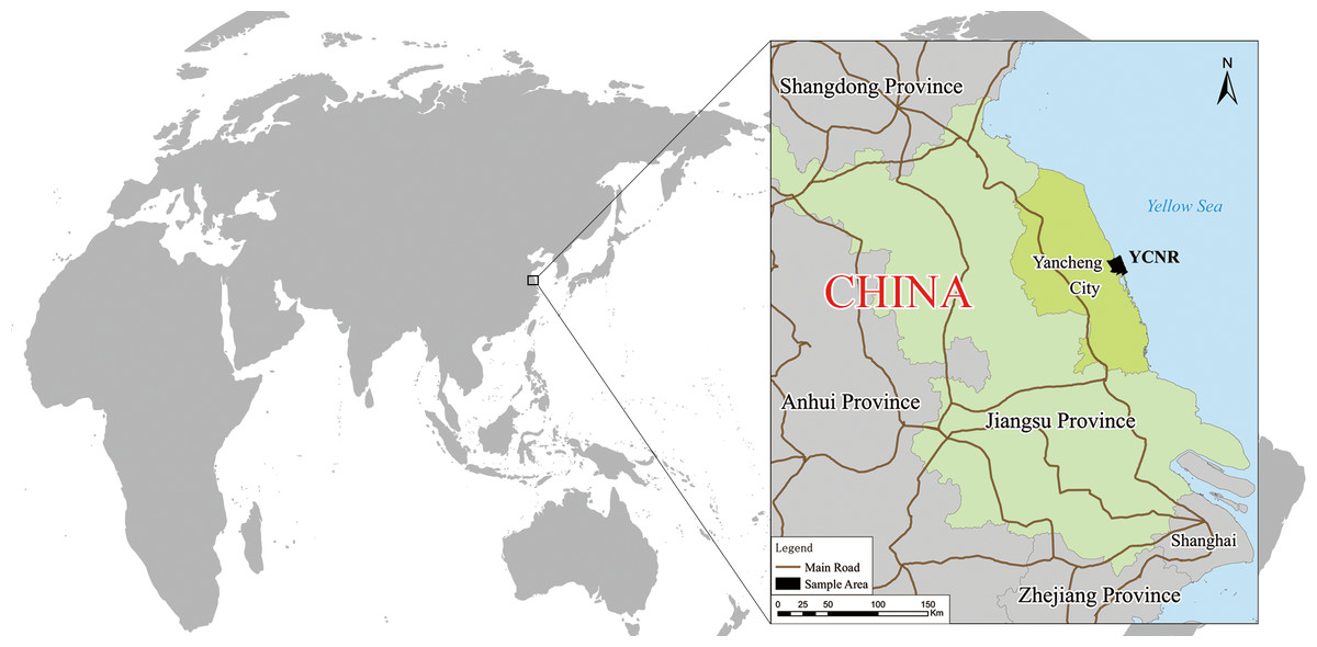
Figure 1: Yancheng coastal natural wetland (YCNR) location in China.
Source and processing of remote-sensing data
To obtain the landscape classification map of the YCNR, we selected these images on the basis of the following criteria: images taken (a) between September and December, when S. alterniflora was grown; (b) under appropriate conditions, such as less than 20% cloud cover; and (c) at low tide, so that S. alterniflora could be seen growing in the intertidal zone. On the basis of the vector boundary of the study area, a remote-sensing image was cropped in ENVI software and enhanced. The FLAASH atmospheric-correction module was used to apply atmospheric corrections to the remote-sensing image. The FLAASH settings are as follows: (1) coordinates of the scene centre point: it was found from the corresponding HDF file; (2) sensor type: Landsat 5, 7 or 8; (3) altitude: the average altitude of the sample area; (4) flight date and time: it is Greenwich mean time, which can be found in the corresponding HDF file; (5) atmospheric model: mid-latitude winter; (7) aerosol model: rural; and we used the default values for the remaining parameters. The geometric-precision-correction module was used to combine the field control point with the image geometry school. The 8 obtained images were visually interpreted. Water, roads and aquaculture ponds were very easy to distinguish. The NDVI threshold was used when interpreting vegetation. The above raw data were obtained from the International Scientific Data Service Centre (http://www.gscloud.cn). On the basis of remote sensing images from 1985, 1990, 1995, 2000, 2005, 2010, 2015, and 2017 (Table 1), we monitored the dynamic changes in typical coastal wetlands, and the combined transition matrix and CA Markov model were analysed for simulation prediction. The images of 2005 and 2007 were from Landsat 7. We fixed the image bands with the landsat_gapfill patch in ENVI software.
| Year | Satellite | Sensor | Acquisition Time | WRS Path | WRS Row | Spatial Resolution | Roll Angle | Cloud Cover | Landsat Scene Identifier |
|---|---|---|---|---|---|---|---|---|---|
| 1985 | Landsat 5 | TM | 24 Sep 1985 01:59:44 | 119 | 037 | 30 m | – | 3% | LT51190371985267HAJ00 |
| 1990 | Landsat 5 | TM | 8 Oct 1990 01:50:08 | 119 | 037 | 30 m | – | 8% | LT51190371990281HAJ00 |
| 1995 | Landsat 5 | TM | 9 Dec 1995 01:31:09 | 119 | 037 | 30 m | – | 1% | LT51190371995343CLT00 |
| 2000 | Landsat 7 | ETM+ | 9 Sep 2000 02:21:17 | 119 | 037 | 30 m | – | 53% | LE71190372000253EDC01 |
| 2005 | Landsat 7 | ETM+ | 26 Nov 2005 02:20:07 | 119 | 037 | 30 m | – | 6% | LE71190372005330EDC00 |
| 2010 | Landsat 7 | ETM+ | 10 Dec 2010 02:23:33 | 119 | 037 | 30 m | – | 1% | LE71190372010344EDC00 |
| 2015 | Landsat 8 | OLI | 13 Oct 2015 02:30:32 | 119 | 037 | 30 m | −0.001 | 0.04% | LC81190372015286 LGN01 |
| 2017 | Landsat 8 | OLI | 5 Dec 2017 02:30:40 | 119 | 037 | 30 m | −0.001 | 0.58% | LC81190372017339 LGN00 |
Model simulation method
The cellular-automaton Markov model method was used for simulation research to reveal the characteristics and regularity of coastal-wetland-landscape succession in the S. alterniflora non-invasion scenario. The Markov model is stochastic and mainly used for the simulation of landscape and land-use changes (Adhikari & Southworth, 2012; Baker, 1989; Tine, Perez & Molowny-Horas, 2019; Yu, He & Pan, 2010). Recent studies have shown that the cellular-automaton Markov model is particularly suitable for the simulation of vegetation succession on a landscape scale in areas not affected by human activity (Sun & Liu, 2014). This model uses the previous time step to simulate the next one, and it can therefore be used to simulate the succession trend of a native ecosystem in a state where S. alterniflora has not invaded.
Cellular automata and the Markov model are both discrete dynamic models of the temporal state. The cellular automaton model has powerful spatial calculation capabilities, but it is not as good as the Markov model in quantitative calculations. The Markov model mainly focuses on predicting the magnitude of change, but it cannot predict the spatial distribution (Zhang, 2012). Combining the cellular automaton model with the Markov model can construct a model that has both the ability of the CA model to simulate the spatial changes of complex systems and the long-term numerical prediction ability of the Markov model.
The optimal parameters of the simulation effect of this study were as follows: step size: 1 year; filter size: 5 × 5; number of iterations: 20; and cell size: 30 m. We tested the accuracy of the model with a kappa coefficient by using the VALIDATE module in IDRISI Selva software; the kappa coefficient was obtained from statistics on the 1995 interpretation result and 1995 native vegetation landscape maps, which quantitatively reflected the accuracy of the model simulation. Simulation-accuracy parameters were tested: the accuracy rate was 0.9152, and the kappa index exceeded 0.8, reflecting the high credibility of the simulation results and indicating that the CA Markov model could be used to simulate the state of S. alterniflora invasion succession of vegetation communities in a typical coastal wetland in Yancheng. More information can be found in Appendix A.
Mean distance of vegetation-type change
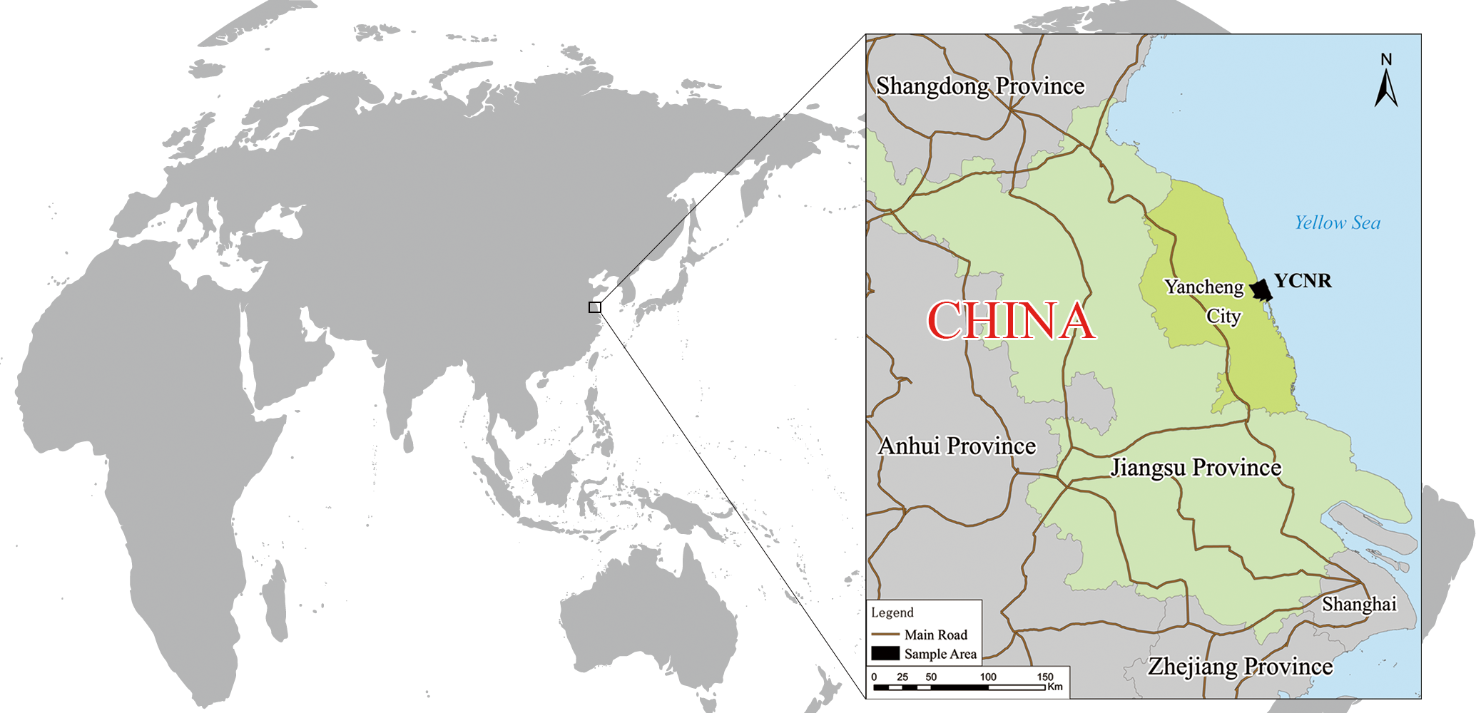
The mean distance is used to indicate a trend of vegetation boundary movement. The following formula was used to calculate the mean distance: (1) where L is the mean distance from the farthest/nearest boundary to the seawall highway; S is the seawall highway, which was used as the reference line, perpendicular to the sea and land direction of the seawall highway; the farthest/nearest boundary of the landscape zone and the seawall highway reference line are areas enclosed by vertical lines of the two; and D is the projected length of the nearest/farthest boundary on the seawall baseline (Fig. 2).
Figure 2: Schematic diagram of mean distance.
S1 is the area enclosed by the nearest boundary and seawall baseline; S2 is the area enclosed by the farest boundary and seawall baseline; D1 is the projected length of the nearest boundary on the seawall baseline; D2 is the projected length of the farthest boundary on the seawall baseline.
Results
Succession characteristics of a native wetland landscape
The transition probability matrix was obtained by analysing the 1985 and 1990 images (Table 2). The native wetland landscape in the YCNR was obtained by the CA-Markov model. Under native vegetation succession, 87.89% of S. salsa still grew in the second year, 11.28% was replaced by P. australis, and 0.83% was degraded to mudflat. Then, 98.02% of P. australis still grew in the second year, 5.98% was degraded to S. salsa, and 0.83% degraded to mudflat.
| S. salsa | P. australis | Mudflat | |
|---|---|---|---|
| S. salsa | 0.8789 | 0.1128 | 0.0083 |
| P. australis | 0.0183 | 0.9802 | 0.0015 |
| Mudflat | 0.0598 | 0.0031 | 0.9370 |
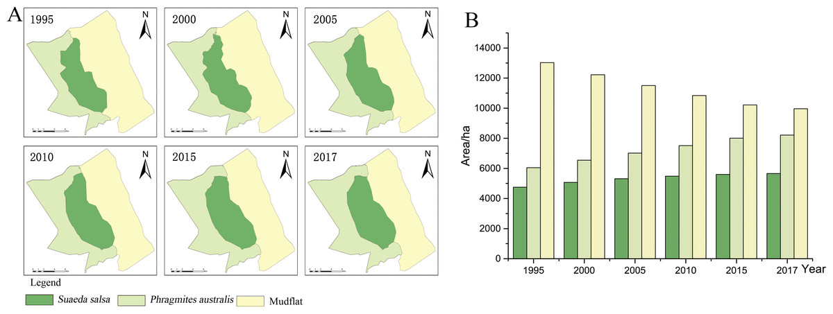
Figure 3: Succession of native vegetation in typical wetlands in YCNR.
(A) The simulation results ranged from 1995 to 2017, which is succession of native vegetation in typical wetlands in YCNR. (B) The area statistics of different vegetation.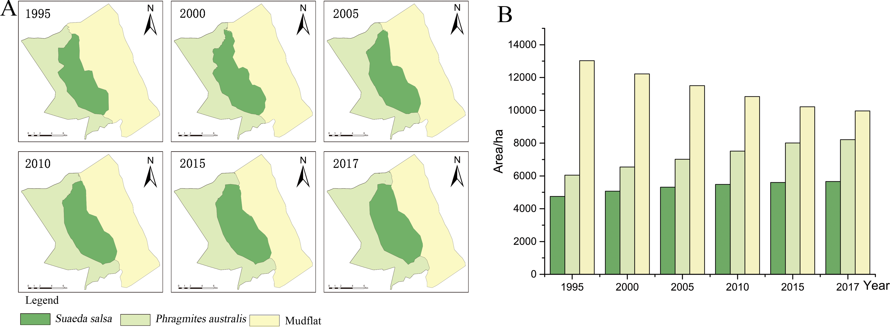
The cellular automaton Markov model simulated the succession of native landscapes without S. alterniflora invasion (Fig. 3). The simulation results showed the succession of native vegetation. The area of native S. salsa increased by 909.41 hectares from 1995 to 2017. The area of native P. australis continued to increase, with an increase of 2157.21 hectares (35.65%). Community succession occurred at all times in the wetlands. A new Suaeda grew on the mudflat, while other Suaeda populations were replaced by P. australis. From 1990 to 1995, 784.70 hectares of new Suaeda bonata grew on the mudflat, while 790.39 hectares of S. salsa was replaced by P. australis. From 1995 to 2000, the 448.26 hectares of mudflat succeeded in becoming S. salsa, and the 534.68 hectares of S. salsa turned into P. australis. From 2000 to 2005, only 30.71 hectares of mudflat succeeded to S. salsa, and 256.58 hectares of S. salsa changed to P. australis. Between 2010 and 2015, only 46.34 hectares of mudflat area was transformed into S. salsa, and 237.11 hectares of S. salsa changed into P. australis.
With a full YCNR landscape structure and a low degree of fragmentation, the centroid may be used to represent a good succession landscape. The native vegetation distribution was roughly strip-shaped with a complete landscape structure and low landscape fragmentation degree. From the land seaward, the vegetation transitioned from P. australis to S. salsa to mudflats. Regarding the change direction (Table 3), P. australis subsided seaward each year. From 1995 to 2017, the centroid moved 877.50 m seaward, and the average seaward speed was 39.89 m/year. The centroid of S. salsa moved seaward. From 1995 to 2017, it moved 1281.10 m seaward with an average speed of 58.23 m/year.
Simulation results (Fig. 4) showed that native P. australis was mainly distributed in the range of 3.3–8.8 km from the seawall, and the average patch bandwidth was 4.6 km. Native S. salsa was mainly distributed in the range of 6.1–11.5 km from the seawall, and the average patch bandwidth was 4.1 km. The maximum distance of P. australis from the seawall baseline moved from the original 14,076.88 m to the land to 11,764.52 m and moved 2323.36 m to the land; the maximum distance from the seawall to the land from the original 12980.36 m moved to the land to 11,816.31 and 1164.05 m.
| Distance (m) | Expansion rate (m/year) | |||||
|---|---|---|---|---|---|---|
| P. australis | S. salsa | Mudflat | P. australis | S. salsa | Mudflat | |
| 1995 | 5079.82 | 7949.92 | 13243.89 | |||
| 37.73 | 75.81 | 41.49 | ||||
| 2000 | 5268.48 | 8328.99 | 13451.33 | |||
| 31.28 | 67.27 | 38.69 | ||||
| 2005 | 5424.88 | 8665.32 | 13644.77 | |||
| 43.32 | 50.79 | 34.91 | ||||
| 2010 | 5641.46 | 8919.29 | 13819.33 | |||
| 45.24 | 44.48 | 31.64 | ||||
| 2015 | 5867.64 | 9141.70 | 13977.54 | |||
| 44.84 | 44.66 | 31.91 | ||||
| 2017 | 5957.32 | 9231.02 | 14041.36 | |||
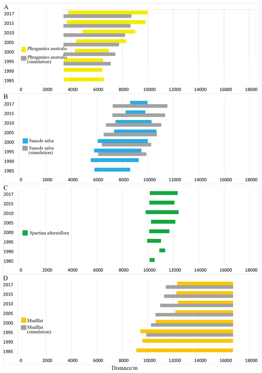
Figure 4: Width distribution of four main landscape types.
Detailed data in Table A1. (A) Width distribution of P. australis; (B) distribution of S. salsa; (C) width distribution of S. alterniflora; (D) width distribution of mudflat.
Impact of S. alterniflora invasion on spatiotemporal succession of natural wetland types
Spatiotemporal succession of wetland landscape types
Table 4 shows the area of each landscape type in eight periods for a typical coastal wetland. As shown in the table, the area of S. salsa first increased and then decreased, the mudflat area decreased, the areas of S. alterniflora and P. australis increased, and the area of water remained basically unchanged. The area of artificial landscapes represented by aquaculture ponds and roads increased, but this increase was small. Specifically, the area of S. salsa increased from 3773.05 hectares in 1985 to 5227.79 hectares in 2000 and then decreased to 992.46 hectares in 2017, with the proportion increasing from 15.83% in 1985 to 21.94% and sharply decreasing to 4.16% in 2017. The area of P. australis increased significantly, from 5038.48 hectares in 1985 to 8571.37 hectares in 2017, accounting for an increase ranging from 21.14% to 36.72%, which was 1.74 times the original area. S. alterniflora increased from 514.53 hectares in 1985 to 3925.46 hectares in 2017, an increase of 662.92%. The mudflat accounted for more than 35% of the entire landscape ecosystem, and the area decreased from 14,424.51 hectares in 1985 to 8,295.04 hectares in 2017, with the proportion falling from 60.53% to 34.81%. The area of aquaculture ponds maintained an increasing trend from 2000 to 2010. The area of roads increased slowly for 27 years, from 61.00 hectares in 1985 to 1,050.98 hectares in 2017.
| 1985 | 1990 | 1995 | 2000 | 2005 | 2010 | 2015 | 2017 | |
|---|---|---|---|---|---|---|---|---|
| S. salsa | 3773.05 | 4584.83 | 4771.35 | 5227.79 | 3385.65 | 2656.16 | 1498.06 | 992.46 |
| P. australis | 5038.48 | 4887.95 | 4765.92 | 3221.19 | 4904.90 | 5602.39 | 8242.41 | 8751.37 |
| S. alterniflora | 214.53 | 211.52 | 680.60 | 2173.89 | 3381.34 | 4318.84 | 3985.08 | 3925.46 |
| Mudflat | 14,424.51 | 13,592.65 | 13,232.36 | 10,213.61 | 8640.78 | 8140.35 | 8417.34 | 8295.04 |
| Water | 318.86 | 492.74 | 328.18 | 545.36 | 813.28 | 445.59 | 504.19 | 472.38 |
| Aquaculture ponds | 2018.31 | 2209.76 | 2261.26 | 252.81 | 342.92 | |||
| Road | 61.00 | 60.82 | 52.07 | 430.31 | 494.83 | 405.87 | 930.70 | 1050.98 |
| Total | 23,830.43 | 23,830.51 | 23830.47 | 23,830.46 | 23,830.54 | 23,830.46 | 23,830.60 | 23,830.60 |
Typical coastal wetlands in Yancheng have P. australis, S. salsa and S. alterniflora as the main landscape types, and the band distribution was obvious. Viewed from a single landscape (Fig. 4), P. australis was mainly distributed on the coast, 3.3–9.9 km from the seawall, with an average width of 4.0 km. From 1985 to 1995, the farthest boundary of P. australis continued to move seaward. Over the course of 32 years, it moved 3,443 m seaward at a speed of 107.6 m/year. The width of the P. australis landscape belt expanded from 3.16 km in 1985 to 6.28 km in 2017.
The landscape of S. salsa was mainly distributed on the coast, 5.8–10.6 km from the seawall baseline, with a mean width of 2.9 km. The nearest boundary of S. salsa moved from 5.8 km seaward in 1985 to 8.6 km in 2017, and the farthest boundary of S. salsa moved from 8.6 to 9.9 km seaward in 1985, with a movement rate of 42.56 m/year. From 1985 to 2000, the width of the S. salsa landscape belt expanded from 2.8 to 3.9 km, with an expansion rate of 75 m/year; from 2000 to 2017, the S. salsa belt width decreased sharply to 1.4 km, with a reduction rate of 151 m/year.
The S. alterniflora patch was mainly distributed 9.8–12.4 km from the seawall baseline. The mean width of the patch was 1.5 km, and the maximum width was 2.6 km. From 1985 to 1990, S. alterniflora was sporadically scattered on the coastal wetlands without banding. From 1985 to 2010, the width of the S. alterniflora patch expanded each year from 0.3 to 2.6 km. From 2010 to 2017, the width of the S. alterniflora patch decreased from 2.6 to 2.1 km.
Impact of S. alterniflora invasion on native landscape succession
S. alterniflora, as an alien species in the YCNR, occupies the living space of native species (Fig. 5). A comparison of the simulation and current situation shows that the area of S. salsa decreased from 5662.05 to 992.46 hectares of the actual area, and the proportion of the reduced area was 82.47%; the P. australis-marsh-wetland area increased from 8208.80 to 8751.37 hectares, accounting for 6.62%. The farthest boundary of S. salsa moved from 11,551.51 m to the land to 9997.24 m, and the farthest boundary moved 1581.27 m to the land and moved 1341.18 m seaward. The average landscape bandwidth of S. salsa also sharply decreased from 4.3 to 1.4 km. S. salsa was forced to contract by receiving stress from both sides, sea and land.
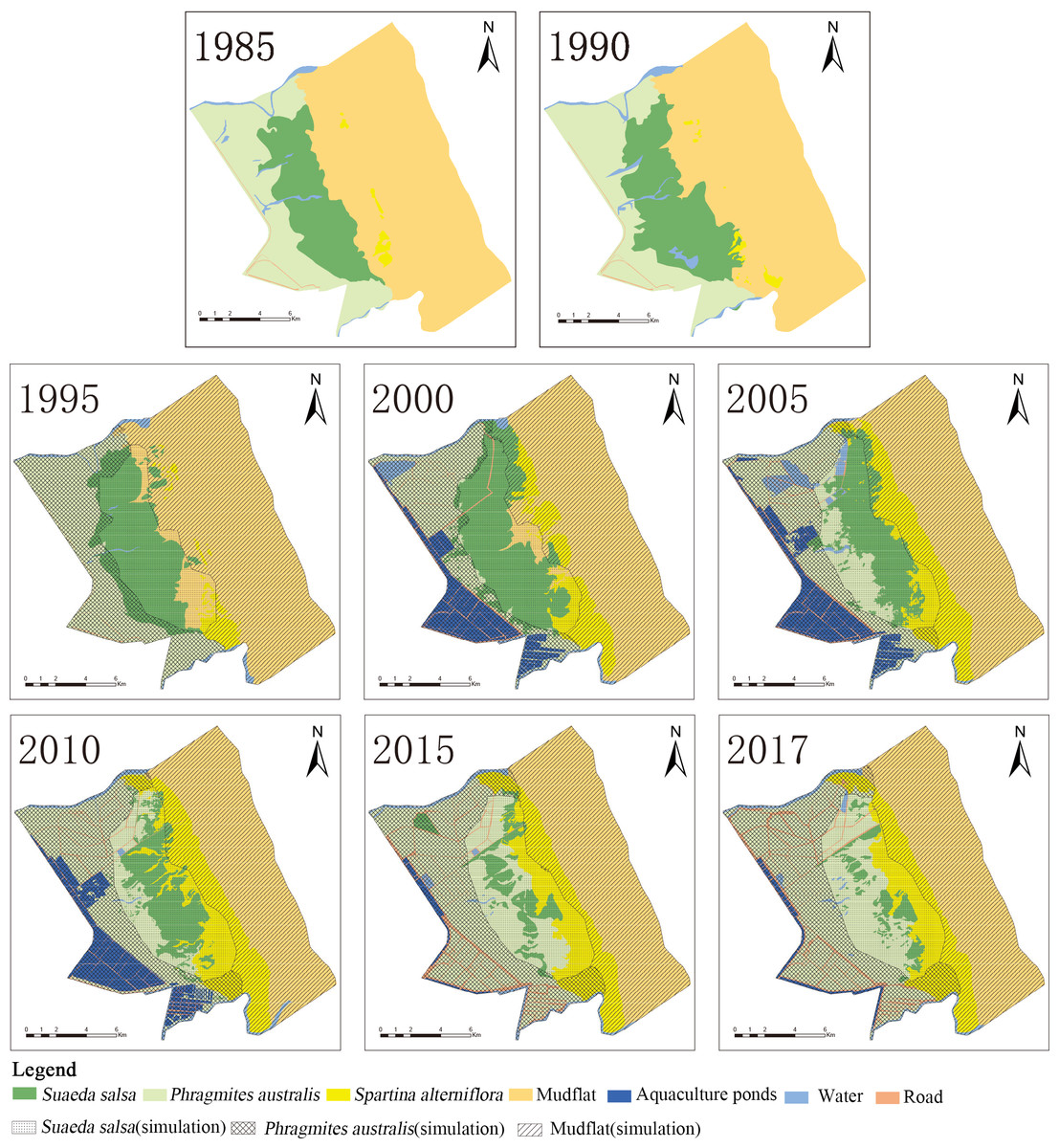
Figure 5: Overlaid map of native vegetation succession and current status.
The detailed data are shown in Table A2. (A) The landscape of YCNR in 1985; (B) the landscape of YCNR in 1990; (C) overlaid map of landscape in 1995; (D) overlaid map of landscape in 2000; (E) is overlaid map of landscape in 2005; (F) overlaid map of landscape in 2010; (G) overlaid map of landscape in 2015; (H) overlaid map of landscape in 2017.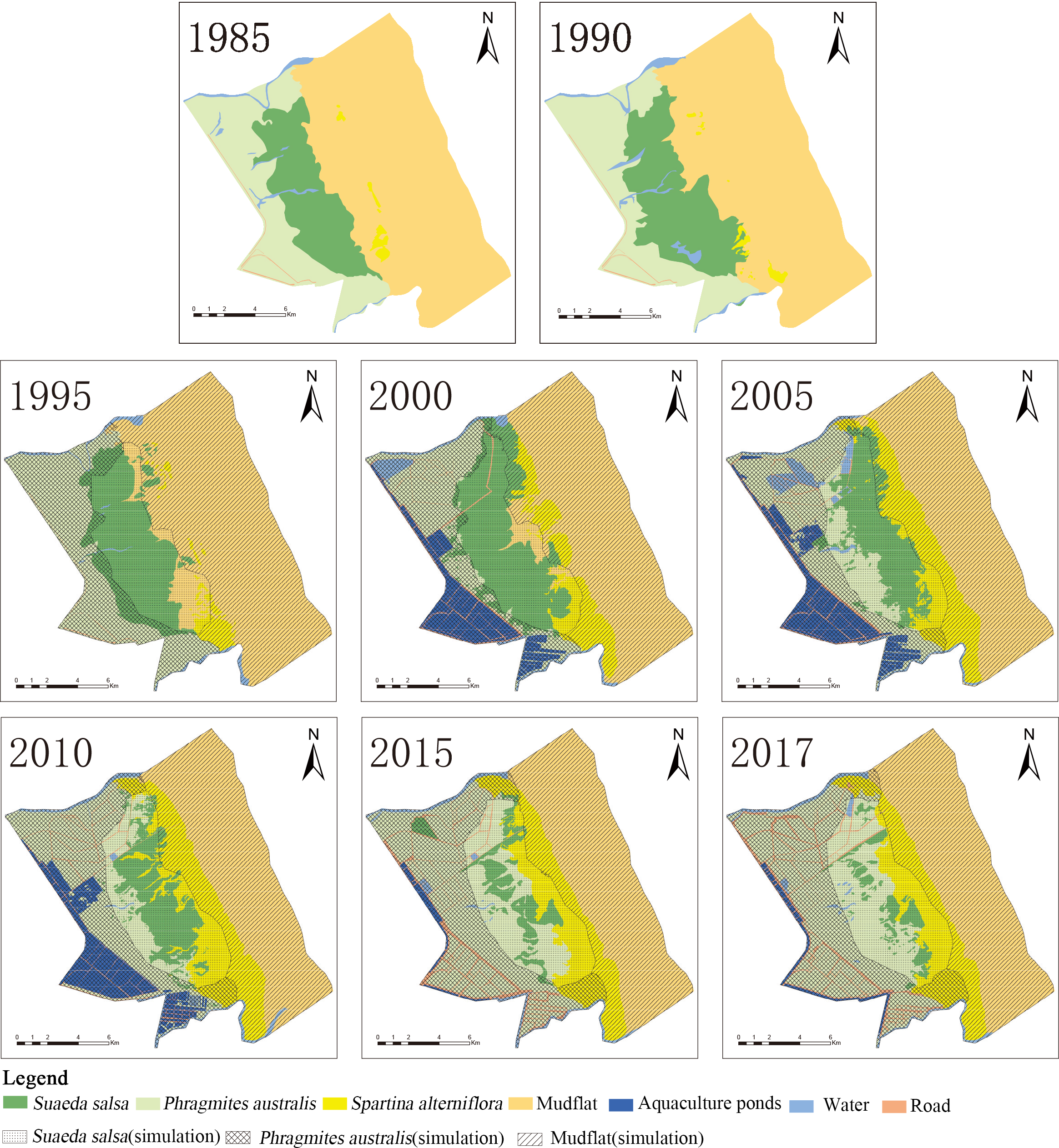
The area of native S. salsa was reduced from 3527 hectares in 1995 to 969 hectares in 2017. The area occupied by P. australis continued to increase from 5 hectares in 1995 to 3,298 hectares in 2017, accounting for an increase of 0.11% from 53.51%. The area occupied by S. alterniflora increased from 167 hectares in 1995 to 1500 hectares in 2017, with an increase of 888.7%. The area occupied by the artificial landscape was less than 100 hectares.
The area of native P. australis increased from 4738 hectares in 1995 to 5720 hectares in 2017. The area occupied by S. alterniflora continued to increase, accounting for an increase from 0.02% in 1995 to 9.73% in 2017. From 2005 to 2017, the area of native P. australis that degraded to S. salsa accounted for less than 3%. The area of native P. australis that developed into artificial landscapes increased to a maximum of 2610 hectares in 2010 and subsequently decreased to 1284 hectares in 2017.
The simulation results showed that, without being affected by S. alterniflora, the farthest/nearest boundaries of the P. australis and S. salsa landscape patches moved seaward, and the average width of the landscape patch expanded (Table 5). The invasion of S. alterniflora affected the structure of the local ecosystem, and the boundary of the near-shore end of P. australis was affected by human activities. It moved 1000–1500 m seaward in 2005 and 2010. The farthest P. australis boundary moved seaward, but before 2000, it was slower than the simulated succession speed; after 2005, it was faster than the simulated succession speed. The farthest P. australis boundary moved seaward faster than the near-land boundary, causing the width of the P. australis landscape patch to increase each year. The two borders of the S. salsa landscape patch were affected by P. australis and S. alterniflora. From 1995 to 2017, the nearest boundary of S. salsa continued to move seaward. From 1995 to 2000, the nearest boundary of S. salsa moved lower than the simulated speed. From 2005 to 2017, the nearest boundary moved seaward increasingly faster than the simulated speed. The speed of the seaward movement of the farthest boundary of the S. salsa landscape patch was lower than the simulated speed. The margins of the two ends of the S. salsa landscape patch were forced to shrink, resulting in a sharp reduction in the width of the S. salsa landscape area.
| Year | Landscape Boundary | Change in Average Width | ||
|---|---|---|---|---|
| Nearest Boundary | Farthest Boundary | |||
| P. australis | 1995 | 16.09 | −598.41 | −614.50 |
| 2000 | 902.61 | −507.58 | −1410.19 | |
| 2005 | 1001.00 | 566.82 | −434.19 | |
| 2010 | 1503.99 | 791.54 | −712.45 | |
| 2015 | 278.58 | 1177.33 | 898.75 | |
| 2017 | 347.04 | 1278.79 | 931.74 | |
| S. salsa | 1995 | −376.57 | −402.07 | −25.50 |
| 2000 | −355.70 | −277.05 | 78.65 | |
| 2005 | 786.14 | −60.76 | −846.90 | |
| 2010 | 724.93 | −785.47 | −1510.39 | |
| 2015 | 1011.10 | −1580.20 | −2591.30 | |
| 2017 | 1345.18 | −1581.27 | −2926.45 | |
| Mudflat | 1995 | −461.73 | 0.75 | 462.48 |
| 2000 | 377.86 | 0.75 | −377.12 | |
| 2005 | 1555.81 | 0.75 | −1555.06 | |
| 2010 | 1386.70 | 0.77 | −1385.93 | |
| 2015 | 966.01 | 0.75 | −965.26 | |
| 2017 | 898.39 | 0.75 | −897.64 | |
Notes:
A boundary move seaward has a positive value and a move to land has a negative value.
Discussion
In recent decades, increasing attention has been paid to the study of coastal zones (An et al., 2007; Gao et al., 2014; Hou, Yu & Lu, 2012). China’s marine economy continues to grow steadily, and the scale of development and utilization activities in coastal areas is expanding rapidly (Liu et al., 2015), but the YCNR has preserved the most complete wetland ecosystem, protecting rare wild animals, such as red-crowned cranes, and their habitats (Cao et al., 2016; Jun et al., 2011). The S. alterniflora invasion severely changed the natural succession law of the native wetland ecosystem in the intertidal zone of the YCNR (Gao et al., 2014; Hou, Yu & Lu, 2012). The understanding of this issue is limited to ecological studies, and it is difficult to understand the problem of the spatial development of succession stages. Using landscape ecology, with the help of remote sensing and GIS, it is possible to accurately explain the interactions and changes between ecosystems from a larger (landscape) macroscale (Gauch, 1982; Jongman, Braak & Tongeren, 1995; Zhang, 2004).
The succession of natural wetlands
Seawall roads, rivers, and oceans make the study area a closed, independent system that induces internal and external drivers of system changes. Soil fertility, population competition and other variables are considered internal driving factors, while human activity disturbance and alien species are considered external driving factors. Landscape changes directly reflect the direction and extent of system changes. The CA-Markov model simulated the natural succession of coastal wetlands with only internal drivers. By comparing the model results with the actual landscape structure, we were able to better understand the impact of external drivers on system changes. The succession model of coastal wetland ecosystems was built using a space-for-time substitution approach (Yao et al., 2009). S. salsa was the pioneer species, taking the lead in occupying the mudflat. Then, P. australis replaced S. salsa, and the area of S. salsa and P. australis continued to increase. This is the law of native vegetation succession. S. salsa and P. australis populations increased in size and area, and the succession direction moved towards the sea. There were no competing species on the east side of S. salsa, and there was sufficient space for growth and nutrition. S. salsa spread and grew, but the soil salinity decreased as the north-south direction approached the inland river. The low-salinity soil environment inhibited the growth of S. salsa. P. australis grew on the west side of S. salsa. P. australis has more advantages in terms of competing with S. salsa for survival space, and S. salsa is gradually being replaced by P. australis.
External driving factors change the succession of the system. Area change can indicate the specific role of the impact factor. The areas of ponds and roads indicate the impact of human activities on the YCNR. From 2000 to 2010, the proportion of artificial landscapes in the area of native P. australis remained at approximately 35% because artificial ponds occupied a large area and kept P. australis near the seawall. In 2013, the protected area implemented the policy of “returning fishing and returning wetness” to stop artificial breeding activities, and the artificial breeding ponds were soon restored to reeds. Human activities mainly affected P. australis and had less effect on S. salsa.
The alien species S. alterniflora was introduced into the YCNR, producing hybrids that were more invasive than their parents (Anttila et al., 1998; Ayres et al., 1999; Daehler & Strong, 1997), competing for indigenous plants (Callaway & Josselyn, 1992; Chen et al., 2004; Daehler & Strong, 1996). S. alterniflora occupied the living space of native vegetation, suggesting that S. alterniflora inhibits the indigenous vegetation, such as common reed and S. salsa.
In the natural state, the average grain size of the surface sediment increases from land to sea, and the sorting becomes better (Alexander et al., 1991; Evans, 1965; Ren, 1986). S. alterniflora is densely distributed, and its stems and leaves have a strong buffering effect on the flow, which can significantly slow the flow velocity, reduce the tidal current transport capacity, and play a role in capturing suspended sediment, thus increasing the sedimentation rate (Frey & Basan, 1978). The results show that there is a negative feedback between the deposition rate and the elevation of the tidal flat. With the silting up of the tidal flat, the inundation time of tidal water is gradually shortened, and salt-tolerant vegetation such as Artemisia halophyte begins to grow on the beach surface, forming salt marsh wetlands. The elevation of the surface layer of the salt marsh wetland increases due to sediment deposition, which leads to a decrease in the water depth during times of tidal inundation, a reduction in suspended solids brought to the salt marsh, and a shortening of the tidal submergence time, which in turn leads to a decrease in the salt marsh deposition rate (Pethick, 1981).
Biological dam
S. alterniflora had spread to the entire coastline in just 20 years. After 2005, the area of S. alterniflora had not increased significantly, and the width remained unchanged. However, the area of S. Suaeda was still rapidly decreasing; the direction of the boundary spread at the far-continent end of S. salsa changed from seaward to landward; the speed of the nearest boundary of S. salsa moving seaward and was higher than that of the simulated case; the speed of the farthest P. australis boundary accelerated towards the sea. The S. alterniflora invasion may indirectly alter the internal conditions of the system, and the biological dam conjecture was proposed (Fig. 6). S. alterniflora spread into flakes in 2000, and the root system of S. alterniflora is thick and dense, which promotes rapid sedimentation and sedimentation (Gleason et al., 1979), changes the terrain of the intertidal zone and prevents the flow of tidal trenches and waterways (Daehler & Strong, 1996). A biological dam was formed in the outermost layer of the coastal wetlands. A biological dam is a hypothetical concept and was composed of S. alterniflora. The thick rhizome accelerated sediment deposition, elevated local topography and changed the ecohydrological mechanism (Millard et al., 2013; Zhao-qing et al., 2020). Biological dams weakened the ecological effects of tides on the YCNR. S. alterniflora was strip-shaped and weakened the energy of the tidal water movement. Substances carried in seawater were deposited on the mudflats in advance, causing the soil salinity of the S. alterniflora zone to increase and reducing the soil salinity of the S. salsa zone, inhibiting the succession of S. salsa seaward. At the same time, the salt moved downward under the action of precipitation, and under the action of runoff, the salt moved to the sea and was deposited at the biological dam. The reduced soil salinity inside the dam was more suitable for the expansion of P. australis populations and inhibited the survival space of S. salsa. The biological dam formed by S. alterniflora weakened the ability of material exchange between the ocean and wetlands. Wetland soil salinity was reduced, making it more suitable for reed growth. The biological dam conjecture is an ideal model, which needs further study and verification. Climate change and marine hydrological impacts were not considered.
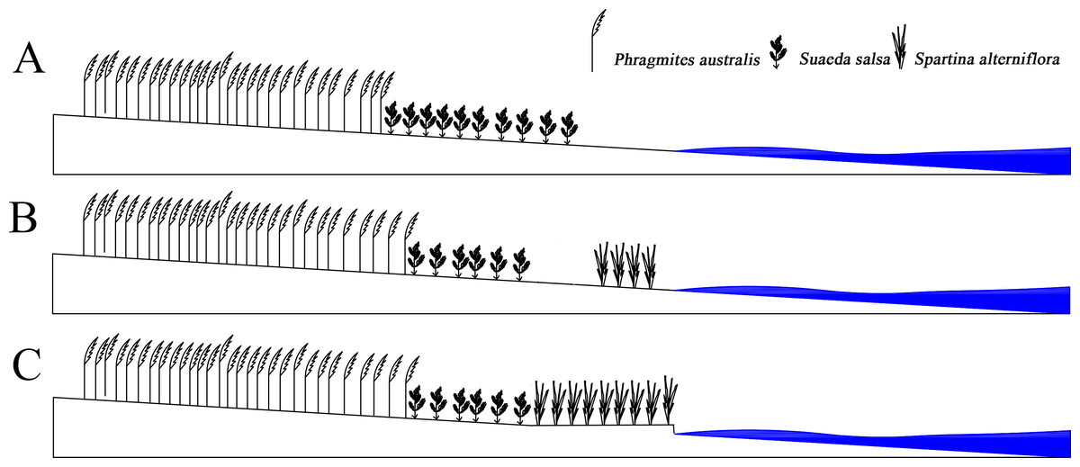
Figure 6: Concept of Biological dam.
(A) shows S. alterniflora has not yet invaded; (B) shows S. alterniflora has just been introduced, and (C) shows that S. alterniflora forms a biological dam.
S. alterniflora was introduced to promote silt protection. However, it was classified as an invasive species. A sustainable control method is urgently needed to effectively protect the ecosystem and prevent the further invasion of S. alterniflora. Effective methods should be studied at the physical, chemical, biological, and ecological levels to inhibit the spread of S. alterniflora and eliminate the harm of alien-species invasions that also change native environmental conditions (e.g., geomorphology, hydrology, soil nutrients). It is particularly important to carry out relevant research to restore a suitable living environment for native species. S. salsa provides food, water, and habitat for rare birds, such as red-crowned cranes. Artificially expanding S. salsa can reduce the harm of species invasion. In addition to knowing the harm posed by a species invasion to an ecosystem, the competition between native species is noteworthy. The S. alterniflora invasion might accelerate P. australis succession, and it is necessary to understand the driving mechanism to protect S. salsa and maintain ecological balance and wetland biodiversity in the tidal flat.
Conclusions
The S. alterniflora invasion is likely to have changed the succession characteristics of the native natural wetland landscape system. According to the CA-Markov model simulation results, the area of P. australis and S. salsa marsh wetlands increased each year when S. alterniflora was not introduced. However, under the influence of S. alterniflora, the area of P. australis marsh-wetland area slowed its spread, and the area of S. salsa marsh wetland decreased each year.
Our results suggest that S. alterniflora invasion changed the original natural wetland landscape succession direction. Without being invaded by S. alterniflora, the P. australis marsh wetland basically did not move in the land section, and the offshore end moved seaward at a speed of 50 m/year; the near-land section of the S. salsa marsh wetland moved seaward at a speed of 34.91 m/year. The offshore section moved seaward at a speed of 51.80 m/year. When the S. alterniflora marsh wetland had an agglomeration effect in 2005, it forced the S. salsa wetland to move toward land and change its succession direction.
S. alterniflora and P. australis inhibit the development of S. salsa. P. australis inhibits the expansion of S. salsa toward land, and S. alterniflora is likely to inhibit the movement of S. salsa seaward.
Supplemental Information
Typical wetland simulation and current state transition matrix in Yancheng
Raw Data
Software ArcMap can be used to access this raw data.