
Estimating the average daily rainfall in Thailand using confidence intervals for the common mean of several delta-lognormal distributions
- Published
- Accepted
- Received
- Academic Editor
- Graciela Raga
- Subject Areas
- Agricultural Science, Statistics, Computational Science, Natural Resource Management, Ecohydrology
- Keywords
- Agriculture, Bayesian approach, MOVER, Natural rainfall, Vague prior, Variance
- Copyright
- © 2021 Maneerat and Niwitpong
- Licence
- This is an open access article distributed under the terms of the Creative Commons Attribution License, which permits unrestricted use, distribution, reproduction and adaptation in any medium and for any purpose provided that it is properly attributed. For attribution, the original author(s), title, publication source (PeerJ) and either DOI or URL of the article must be cited.
- Cite this article
- 2021. Estimating the average daily rainfall in Thailand using confidence intervals for the common mean of several delta-lognormal distributions. PeerJ 9:e10758 https://doi.org/10.7717/peerj.10758
Abstract
The daily average natural rainfall amounts in the five regions of Thailand can be estimated using the confidence intervals for the common mean of several delta-lognormal distributions based on the fiducial generalized confidence interval (FGCI), large sample (LS), method of variance estimates recovery (MOVER), parametric bootstrap (PB), and highest posterior density intervals based on Jeffreys’ rule (HPD-JR) and normal-gamma-beta (HPD-NGB) priors. Monte Carlo simulation was conducted to assess the performance in terms of the coverage probability and average length of the proposed methods. The numerical results indicate that MOVER and PB provided better performances than the other methods in a variety of situations, even when the sample case was large. The efficacies of the proposed methods were illustrated by applying them to real rainfall datasets from the five regions of Thailand.
Introduction
Approximately 82.2% of Thailand’s cultivated land area depends on natural rainfall (Supasod, 2006), thereby indicating its importance for Thai agriculture. However, it is a natural phenomenon with a significant level of uncertainty that can cause natural disasters such as droughts, floods, and landslides. In many countries around the world, extreme rainfall events have been increasing in frequency and duration. On December 5, 2017, Storm Desmond led to heavy rainfall causing flooding in northern England, Southern Scotland, and Ireland (Otto & Oldenborgh, 2017). On July 6–7, 2018, extreme rainfall events such as floods and landslides affected over 5,000 houses, and approximately 1.9 million people in Japan were evacuated from the at-risk area (Oldenborgh, 2018). In mid-September 2019, the amount of rainfall was extreme during Tropical Storm Imelda in Southeast Texas, USA, where over 1,000 people were affected by large-scale flooding and there were five deaths (Oldenborgh et al., 2019). Thus, it is necessary to assess how rainfall varies in each region of a country on a daily basis. Due to the climate pattern and meteorological conditions, Thailand is commonly separated into five regions: northern, northeastern, central, eastern, and southern. The rainfall in each region varies widely due to both location and seasonality. Importantly, Thailand’s rainfall data include many zeros with probability δ > 0 and positive right-skewed data following a lognormal distribution for the remainder of the probability. Thus, applying a delta-lognormal distribution (Aitchison, 1955) is appropriate.
The mean is a measure of the center of a set of observations (Casella & Berger, 2002) that can be used in statistical inference, while functions of the mean such as the ratio or difference between two means can also be used. These parameters have been applied in many research areas, such as medicine, fish stocks, pharmaceutics, and climatology. For example, they have been used for hypothesis testing of the effect of race on the average medical costs between African American and Caucasian patients with type I diabetes (Zhou, Gao & Hui, 1997), to estimate the mean charges for diagnostic tests on patients with unstable chronic medical conditions (Zhou & Tu, 2000; Tian, 2005; Tian & Wu, 2007; Li, Zhou & Tian, 2013), to estimate the maximum alcohol concentration in men in an alcohol interaction study (Tian & Wu, 2007; Krishnamoorthy & Oral, 2015), to estimate the mean red cod density around New Zealand as an indication of fish abundance (Fletcher, 2008; Wu & Hsieh, 2014), and to estimate the mean of the monthly rainfall totals to compare rainfall in Bloemfontein and Kimberley in South African (Harvey & van der Merwe, 2012).
In practice, the mean has been widely used in many fields, as mentioned before. When independent samples are recorded from several situations, then the common mean is of interest when studying more than one population. Many researchers have investigated methods for constructing confidence interval (CIs) for the common mean of several distributions. For example, Fairweather (1972) proposed a linear combination of Student’s t to construct CIs for the common mean of several normal distributions. Jordan & Krishnamoorthy (1996) solved the problem of CIs for the common mean under unknown and unequal variances based on Student’s t and independent F variables from several normal populations. Krishnamoorthy & Mathew (2003) presented the generalized CI (GCI) and compared it with the CIs constructed by Fairweather (1972), and Jordan & Krishnamoorthy (1996). Later, Lin & Lee (2005) developed a GCI for the common mean of several normal populations. Tian & Wu (2007) provided CIs for the common mean of several lognormal populations using the generalized variable approach, which was shown to be consistently better than the large sample (LS) approach. Lin & Wang (2013) studied the modification of the quadratic method to make inference via hypothesis testing and interval estimation for several lognormal means. Krishnamoorthy & Oral (2015) proposed the method of variance estimates recovery (MOVER) approach for the common mean of lognormal distributions.
As mentioned earlier, many researchers have developed CIs for the common mean of several normal and lognormal distributions. However, there has not yet been an investigation of statistical inference using the common mean of several delta-lognormal distributions. Since the common mean is used to study more than one population, the average precipitation in the five regions in Thailand can be estimated using it as there is an important need to estimate the daily rainfall trends in these regions. Furthermore, the daily rainfall records from the five regions in Thailand satisfy the assumptions for a delta-lognormal distribution. Herein, CIs for the common mean of several delta-lognormal models based on the fiducial GCI (FGCI), LS, MOVER, parametric bootstrap (PB), and highest posterior density (HPD) intervals based on Jeffreys’ rule (HPD-JR) and normal-gamma-beta (HPD-NGB) priors are proposed. The outline of this article is as follows. The ideas behind the proposed methods are detailed in the Methods section. Numerical computations are reported in ‘Simulation Studies and Results’. In ‘An Empirical Application’, the daily natural rainfall records of the five regions in Thailand are used to illustrate the efficacy of the methods. Finally, the paper is ended with a discussion and conclusions.
Methods
Let Wij = (Wi1, Wi2, …, Wini) be random samples drawn from a delta-lognormal distribution, for i = 1, 2, …, k and j = 1, 2, .., ni. There are three parameters in this distribution: the mean μi, variance and the probability of obtaining a zero observation δi. The distribution of Wij is given by (1) where is a lognormal distribution function, denoted as such that . The number of zeros has a binomial distribution . The population mean of Wij is given by (2)
The unbiased estimates of , and δi are , , and , respectively, where ni = ni(0) + ni(1); . Suppose that the delta-lognormal mean in Eq. (2) for all k populations are the same, then according to Tian & Wu (2007) and Krishnamoorthy & Oral (2015), the common delta-lognormal mean is defined as (3)
For the ith sample, the estimates of ϑi are which contains the unbiased estimates , and . According to Longford (2009), the expected value of is derived as
(4) (5) where as ni → ∞, and E[exp(ciYi)] = (1 − 2ci)−l∕2; and , . If , then we can obtain that
(6)
According to Aitchison & Brown (1963), the Aitchison estimate of ϑi is expressed as (7) where ψa(b) is a Bessel function defined as (8)
To investigate the unbiased estimate , the expected value is
According to Shimizu & Iwase (1981), the uniformly minimum variance unbiased (UMVU) estimate of ϑi is (9) where and ; (10)
From Kunio (1983), is obtained, then (11)
where E(ni(1)) = ni(1 − δi). The asymptotic variance of is given by
(12) Actually, such that and are the unbiased estimates of ϑi under different ideas, although their variances are the same i.e., . Using , and from the samples, the estimated delta-lognormal mean and variance of are obtained. The following methods are the detailed construction of the CIs for the common delta-lognormal mean.
Fiducial generalized confidence interval
Fiducial inference was introduced by Fisher (1930). Fisher’s fiducial argument was used to develop a generalized fiducial recipe that could be extended to the application of fiducial ideas (Hannig, 2009). The concept of the fiducial interval has been advanced by the idea of the generalized pivotal quantity (GPQ) such that it is directly used to apply for generalized inference. Later, Hannig, Iyer & Patterson (2006) argued that a subclass of GPQs, the fiducial GPQ (FGPQ), provides a framework that shows the connection between a distribution and a parameter. Recall that and are the independent random variables. The structure functions of and are (13) which are the function of Vi and Ui, respectively, where Vi ∼ N(0, 1) and . Given the observed values, the estimates and can be obtained, and the unique solution of becomes (14) The respective FGPQs of μi and are (15) (16) where and are independent copies of Vi and Ui, respectively. Hasan & Krishnamoorthy (2018) developed the FGPQ of δi using a beta distribution as ; αi = ni(1) + 0.5 and βi = ni(0) + 0.5. The FGPQ of ϑ based on k individual samples is (17) where , , and . Thus, the 100(1 − ζ)% FGCI for ϑ is (18) where Gϑ(ζ) denotes the ζth percentiles of Gϑ. Algorithm 1 shows the computational steps for obtaining the FGCI.
Algorithm 1: FGCI
-
Generate Vi ∼ N(0, 1) and are independent.
-
Compute the FGPQs Gμi, and .
-
Compute Gwi and Gϑi leading to obtain Gϑ.
-
Repeat steps 1-3, a number of times, m = 2500, compute 95%FGCI for ϑ, as given in Eq. (18).
Large sample interval
Recall that the Aitchitson estimator is and the variance of is . The approximated variance is obtained by replacing , and . The pooled estimate of ϑi is given by (19) where . Hence, the 100(1 − ζ)% LS interval for ϑ is obtained as (20) where zζ denotes the ζth percentiles of standard normal N(0, 1). The LS interval can be estimated easily via ‘Algorithm 2’.
Algorithm 2: LS
-
Compute and .
-
Compute .
-
Compute 95%LS interval for ϑ, as given in Eq. (20).
Method of variance estimates recovery
This method produces a closed-form CI that is easy to compute. For this reason, the MOVER CI for the common delta-lognormal mean is considered for k individual random samples. The MOVER for a linear combination of ϑi; i=1 , 2, …, k is as follows. Let be independent unbiased estimators of ϑ1, ϑ2, …, ϑk, respectively. In addition, let [li, ui] stand for the 100(1 − ζ)%CI for ϑi. According to Krishnamoorthy & Oral (2015), the 100(1 − ζ)%MOVER for is given by (21) where and . Next, the closed-form CIs for ϑi are needed to construct MOVER for ϑ. Thus, ϑi is log-transformed as (22) where . Let , and and be the unbiased estimates of μi, , and δi, respectively. The MOVER for a single delta-lognormal mean presented by Hasan & Krishnamoorthy (2018), the MOVER for ϑi is given by (23) where (24) Note that both , and are independent random variables. According to Krishnamoorthy & Oral (2015), the 100(1 − ζ)% MOVER interval for ϑ is (25) where . ‘Algorithm 3’ describes the steps to construct the MOVER interval.
Algorithm 3: MOVER
Parametric Bootstrap
This is developed from the parametric bootstrap on the common mean of several heterogeneous log-normal distributions, proposed by Malekzadeh & Kharrati-Kopaei (2019). The delta-lognormal mean is transformed by taking the logarithm as (26)
The likelihood of is (27) which enables obtaining the maximum likelihood estimates of lnϑ and as (28) where and ; . If δi = 0, then it becomes the common lognormal mean (see Krishnamoorthy & Oral (2015) for a detailed explanation). By applying central limit theorem, we obtain such that . It is well-known that , and are independent random variables for which , and are obtained, respectively. Let so that we can write . It can be seen that the distribution of T is complicated, possibly depending on nuisance parameters and δi, but not on lnϑ. Thus, the exact distribution of T is unknown in practice, and so we propose the PB pivotal variable corresponding to TPB as (29) where , , , and , , and . Note that , , and are the observed values of , , and , respectively, from random sampling with replacement based on the bootstrap approach. Thus, the 100(1 − ζ)% PB interval for ϑ is given by (30) where denotes the (1 − ζ)th percentile of distribution of TPB. The PB interval can be constructed as shown in ‘Algorithm 4’.
Algorithm 4: PB
-
Compute , and leading to obtain .
-
Compute and .
-
Generate , and leading to compute .
-
Repeat steps 1-3, a number of time m = 2500, compute TPB to obtain .
-
Compute 95%PB interval for ϑ, as given in Eq. (30).
Highest posterior density intervals
The HPD interval is constructed from the posterior distribution, as defined by Box & Tiao (1973). Note that the prior of ϑi is updated with its likelihood function thereby obtaining the posterior distribution based on the Bayesian approach. Recall that , then the likelihood is given by (31)
For k individual samples, Miroshnikov, Wei & Conlon (2015) described the pooled independent sub-posterior samples toward the joint posterior distributions ϑ are combined using weighted averages as follows: (32) where are the posterior samples of ϑi, for i = 1, 2, …, k. The inverse of the sample variance is used to weight the posterior based on the ith samples is denoted as . Different priors have been developed for estimating the common delta-lognormal mean, two of which are derived in the following subsections.
Jeffreys’ rule prior
Harvey & van der Merwe (2012) defined this prior as (33) which is combined with the likelihood Eq. (34) to obtain the posterior of ϑ as (34) This leads to obtaining the marginal posterior distributions of μi, and δi as (35)
The pooled posterior of ϑ is weighted by its inversely estimated variance as follows: (36) where
.
From Eq. (36), the 100(1 − ζ)%HPD-based Jeffreys’ rule prior (HPD-JR) for ϑ is constructed as follows:
Normal-gamma-beta prior
Maneerat, Niwitpong & Niwitpong (2020) proposed a HPD based on the normal-gamma prior for the ratio of delta-lognormal variances that worked better than the HPD-JR of Harvey & van der Merwe (2012). Suppose that Y = lnW be a random variable of normal distribution with mean μ = (μ1, μ2, …, μk) and precision λ = (λ1, λ2, …, λk) where W ∼ LN(μ, λ) and . The HPD-based normal-gamma-beta prior (HPD-NGB) of ϑ = (μi, λi, δi)′ is defined as (37) where (μi, λi) follows a normal-gamma distribution, and δi follows a beta distribution, denoted as (μi, λi) ∼ NG(μi, λi|μ, ki(0) = 0, αi(0) = − 1∕2, βi(0) = 0) and δi ∼ beta(1∕2, 1∕2), respectively. When the the prior Eq. (37) is combined with the likelihood Eq. (34), then the posterior density of ϑ becomes (38) which can be integrated out to obtain the marginal posterior distributions of μi, λi and δi as follows: (39) where df = 2 (ni(1) − 1) and . Similarly, the pooled posterior of ϑ is given by (40) where .
Hence, the 100(1 − ζ)%HPD-HGB for ϑ is constructed in Eq. (40). ‘Algorithm 5’ details the steps to construct the HPD-JR and HPD-NGB.
Algorithm 5: HPD-JR and HPD-NGB
-
Compute , and .
-
Generate the posterior densities of μi, and δi based-Jeffreys’ rule (JR) and normal-gamma-beta (NGB) priors, as given in Eq. (35) and Eq. (39), respectively.
-
Compute the pooled posterior of ϑ based on JR and NGB priors, as given in Eq. (36) and Eq. (40), respectively.
-
Compute 95%HPD-JR and HPD-NGB for ϑ, defined by Box & Tiao (1973).
Simulation Studies and Results
The performances of the CIs were assessed by comparing their coverage probabilities (CPs) and average length (ALs) using Monte Carlo simulation. The best-performing CI is the one where the CP is closest to or greater than the nominal confidence level 1 − ζ while also having an AL with the narrowest width. The CIs for the common delta-lognormal mean constructed using FGCI, LS, MOVER, PB, HPD-JR, and HPD-NGB were assessed in the study, the parameter settings for which are provided in Table 1. The number of generated random samples was fixed at M = 5000. For FGCI, the number of FGPQs was Q = 2500 for each set of 5,000 random samples. ‘Algorithm 6’ shows the computational steps to estimate the CP and AL performances of all of the methods.
| Scenarios | (n1, …, nk) | (δ1, …, δk) | |
|---|---|---|---|
| k = 2 | |||
| 1–9 | (302) | (0.1,0.2), (0.2,0.5), (0.3,0.7) | (1,2), (2,4), (3,5) |
| 10–18 | (30,50) | (0.1,0.2), (0.2,0.5), (0.3,0.7) | (1,2), (2,4), (3,5) |
| 19–27 | (502) | (0.1,0.2), (0.2,0.5), (0.3,0.7) | (1,2), (2,4), (3,5) |
| 28–36 | (50,100) | (0.1,0.2), (0.2,0.5), (0.3,0.7) | (1,2), (2,4), (3,5) |
| 37–45 | (1002) | (0.1,0.2), (0.2,0.5), (0.3,0.7) | (1,2), (2,4), (3,5) |
| k = 5 | |||
| 46–54 | (305) | (0.05, 0.12, 0.22), (0.22, 0.43), (0.52, 0.73) | (12, 23), (22, 33), (32, 53) |
| 55–63 | (302, 503) | (0.05, 0.12, 0.22), (0.22, 0.43), (0.52, 0.73) | (12, 23), (22, 33), (32, 53) |
| 64–72 | (302, 502, 100) | (0.05, 0.12, 0.22), (0.22, 0.43), (0.52, 0.73) | (12, 23), (22, 33), (32, 53) |
| 73–81 | (30, 502, 1002) | (0.05, 0.12, 0.22), (0.22, 0.43), (0.52, 0.73) | (12, 23), (22, 33), (32, 53) |
| 82–90 | (505) | (0.05, 0.12, 0.22), (0.22, 0.43), (0.52, 0.73) | (12, 23), (22, 33), (32, 53) |
| 91–99 | (502, 1003) | (0.05, 0.12, 0.22), (0.22, 0.43), (0.52, 0.73) | (12, 23), (22, 33), (32, 53) |
| 100–108 | (1005) | (0.05, 0.12, 0.22), (0.22, 0.43), (0.52, 0.73) | (12, 23), (22, 33), (32, 53) |
| k = 10 | |||
| 109–114 | (305, 505) | (0.15, 0.25), (0.25, 0.55) | (15, 25), (25, 45), (35, 55) |
| 115–120 | (303, 503, 1004) | (0.15, 0.25), (0.25, 0.55) | (15, 25), (25, 45), (35, 55) |
| 121–126 | (505, 1005) | (0.15, 0.25), (0.25, 0.55) | (15, 25), (25, 45), (35, 55) |
Notes:
Note: (305) stands for (30, 30, 30, 30, 30).
| Scenarios | CP | AL | ||||||||||
|---|---|---|---|---|---|---|---|---|---|---|---|---|
| FG | LS | MO | PB | HJ | HN | FG | LS | MO | PB | HJ | HN | |
| k = 2 | ||||||||||||
| 1 | 0.959 | 0.897 | 0.967 | 0.994 | 0.916 | 0.941 | 1.556 | 1.296 | 2.005 | 2.324 | 1.353 | 1.436 |
| 2 | 0.958 | 0.857 | 0.947 | 0.996 | 0.924 | 0.941 | 5.169 | 3.770 | 7.287 | 8.631 | 4.186 | 4.335 |
| 3 | 0.963 | 0.821 | 0.959 | 0.996 | 0.919 | 0.932 | 13.088 | 8.675 | 23.312 | 22.883 | 9.905 | 10.220 |
| 4 | 0.962 | 0.886 | 0.978 | 0.995 | 0.917 | 0.939 | 1.487 | 1.211 | 2.181 | 2.155 | 1.247 | 1.386 |
| 5 | 0.953 | 0.832 | 0.962 | 0.995 | 0.913 | 0.922 | 4.875 | 3.487 | 9.881 | 7.818 | 3.811 | 4.066 |
| 6 | 0.951 | 0.793 | 0.971 | 0.991 | 0.901 | 0.912 | 12.311 | 7.740 | 37.615 | 21.129 | 8.875 | 9.378 |
| 7 | 0.961 | 0.829 | 0.972 | 0.982 | 0.920 | 0.940 | 1.511 | 1.095 | 3.968 | 2.173 | 1.224 | 1.406 |
| 8 | 0.950 | 0.778 | 0.974 | 0.995 | 0.900 | 0.911 | 4.821 | 3.123 | 293.620 | 7.649 | 3.566 | 3.916 |
| 9 | 0.939 | 0.725 | 0.973 | 0.988 | 0.866 | 0.887 | 13.159 | 7.067 | 8.0e4 | 23.632 | 8.680 | 9.419 |
| 10 | 0.960 | 0.900 | 0.965 | 0.992 | 0.915 | 0.941 | 1.503 | 1.249 | 1.936 | 2.225 | 1.362 | 1.395 |
| 11 | 0.961 | 0.848 | 0.941 | 0.992 | 0.924 | 0.940 | 5.128 | 3.712 | 6.765 | 8.667 | 4.298 | 4.368 |
| 12 | 0.965 | 0.819 | 0.952 | 0.998 | 0.919 | 0.931 | 12.297 | 8.382 | 20.057 | 21.597 | 9.819 | 9.894 |
| 13 | 0.960 | 0.896 | 0.977 | 0.992 | 0.917 | 0.942 | 1.366 | 1.147 | 1.909 | 2.004 | 1.203 | 1.271 |
| 14 | 0.961 | 0.851 | 0.964 | 0.996 | 0.916 | 0.931 | 4.593 | 3.422 | 7.236 | 7.458 | 3.761 | 3.889 |
| 15 | 0.949 | 0.790 | 0.958 | 0.994 | 0.894 | 0.905 | 11.116 | 7.517 | 22.293 | 19.310 | 8.507 | 8.718 |
| 16 | 0.963 | 0.860 | 0.972 | 0.974 | 0.928 | 0.943 | 1.354 | 1.033 | 2.141 | 1.928 | 1.155 | 1.257 |
| 17 | 0.952 | 0.803 | 0.976 | 0.992 | 0.900 | 0.917 | 4.397 | 3.048 | 10.772 | 6.889 | 3.418 | 3.630 |
| 18 | 0.940 | 0.737 | 0.968 | 0.989 | 0.872 | 0.889 | 11.065 | 6.663 | 43.755 | 19.011 | 7.903 | 8.247 |
| 19 | 0.961 | 0.914 | 0.966 | 0.992 | 0.921 | 0.946 | 1.153 | 1.009 | 1.382 | 1.696 | 1.043 | 1.076 |
| 20 | 0.965 | 0.895 | 0.946 | 0.991 | 0.938 | 0.949 | 3.668 | 2.924 | 4.309 | 5.981 | 3.178 | 3.229 |
| 21 | 0.962 | 0.863 | 0.952 | 0.996 | 0.930 | 0.940 | 8.747 | 6.665 | 11.805 | 14.651 | 7.272 | 7.395 |
| 22 | 0.958 | 0.910 | 0.978 | 0.985 | 0.919 | 0.944 | 1.091 | 0.945 | 1.414 | 1.555 | 0.945 | 1.031 |
| 23 | 0.965 | 0.883 | 0.969 | 0.996 | 0.926 | 0.937 | 3.336 | 2.695 | 4.578 | 5.204 | 2.811 | 2.950 |
| 24 | 0.961 | 0.840 | 0.972 | 0.995 | 0.921 | 0.928 | 7.887 | 5.987 | 13.164 | 12.757 | 6.338 | 6.605 |
| 25 | 0.969 | 0.868 | 0.980 | 0.958 | 0.930 | 0.953 | 1.120 | 0.866 | 1.610 | 1.503 | 0.937 | 1.070 |
| 26 | 0.954 | 0.839 | 0.970 | 0.997 | 0.916 | 0.926 | 3.208 | 2.433 | 6.544 | 4.735 | 2.621 | 2.830 |
| 27 | 0.946 | 0.773 | 0.970 | 0.992 | 0.893 | 0.903 | 7.803 | 5.443 | 26.105 | 12.382 | 6.011 | 6.376 |
| 28 | 0.958 | 0.912 | 0.972 | 0.979 | 0.916 | 0.947 | 1.119 | 0.952 | 1.397 | 1.615 | 1.054 | 1.051 |
| 29 | 0.956 | 0.872 | 0.921 | 0.958 | 0.927 | 0.943 | 3.745 | 2.836 | 4.238 | 6.098 | 3.338 | 3.330 |
| 30 | 0.961 | 0.846 | 0.937 | 0.987 | 0.925 | 0.936 | 8.488 | 6.274 | 10.833 | 13.991 | 7.332 | 7.320 |
| 31 | 0.962 | 0.927 | 0.985 | 0.978 | 0.919 | 0.949 | 0.984 | 0.876 | 1.322 | 1.433 | 0.908 | 0.929 |
| 32 | 0.960 | 0.880 | 0.958 | 0.992 | 0.925 | 0.940 | 3.214 | 2.618 | 4.169 | 5.150 | 2.818 | 2.860 |
| 33 | 0.958 | 0.838 | 0.960 | 0.994 | 0.910 | 0.925 | 7.360 | 5.744 | 10.824 | 12.105 | 6.256 | 6.279 |
| 34 | 0.963 | 0.888 | 0.977 | 0.922 | 0.938 | 0.954 | 0.975 | 0.785 | 1.322 | 1.352 | 0.876 | 0.922 |
| 35 | 0.958 | 0.860 | 0.971 | 0.995 | 0.917 | 0.929 | 2.915 | 2.343 | 4.321 | 4.424 | 2.486 | 2.586 |
| 36 | 0.951 | 0.820 | 0.973 | 0.995 | 0.901 | 0.916 | 6.726 | 5.103 | 11.951 | 10.823 | 5.511 | 5.626 |
| 37 | 0.957 | 0.935 | 0.960 | 0.970 | 0.927 | 0.948 | 0.802 | 0.722 | 0.923 | 1.168 | 0.743 | 0.753 |
| 38 | 0.955 | 0.916 | 0.926 | 0.953 | 0.942 | 0.948 | 2.442 | 2.044 | 2.541 | 3.935 | 2.220 | 2.219 |
| 39 | 0.957 | 0.888 | 0.939 | 0.981 | 0.937 | 0.945 | 5.608 | 4.594 | 6.295 | 9.049 | 4.984 | 4.998 |
| 40 | 0.961 | 0.942 | 0.975 | 0.957 | 0.924 | 0.954 | 0.740 | 0.679 | 0.911 | 1.062 | 0.659 | 0.702 |
| 41 | 0.961 | 0.920 | 0.960 | 0.988 | 0.933 | 0.950 | 2.199 | 1.925 | 2.558 | 3.401 | 1.958 | 2.012 |
| 42 | 0.955 | 0.875 | 0.960 | 0.994 | 0.925 | 0.931 | 4.976 | 4.209 | 6.298 | 7.813 | 4.318 | 4.439 |
| 43 | 0.967 | 0.909 | 0.980 | 0.863 | 0.937 | 0.960 | 0.773 | 0.625 | 0.972 | 1.012 | 0.659 | 0.743 |
| 44 | 0.960 | 0.896 | 0.970 | 0.993 | 0.928 | 0.939 | 2.076 | 1.750 | 2.684 | 3.013 | 1.788 | 1.921 |
| 45 | 0.952 | 0.835 | 0.970 | 0.996 | 0.908 | 0.914 | 4.683 | 3.786 | 7.007 | 7.008 | 3.952 | 4.182 |
Notes:
- FG
-
fiducial generalized confidence interval
- MO
-
method of variance estimates
- HJ
-
HPD-based Jeffreys’ rule prior
- HPD-JR
-
HN, HPD-based normal-gamma-beta prior
Bold denoted as the best-performing method each case.
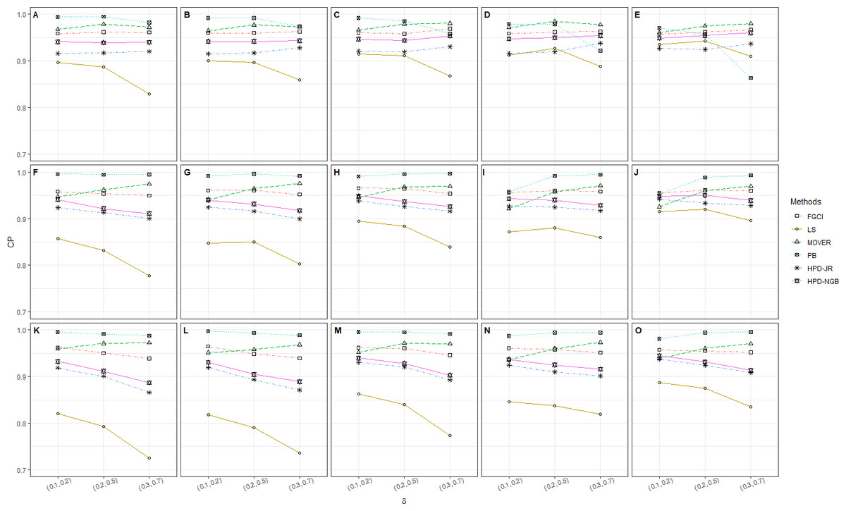
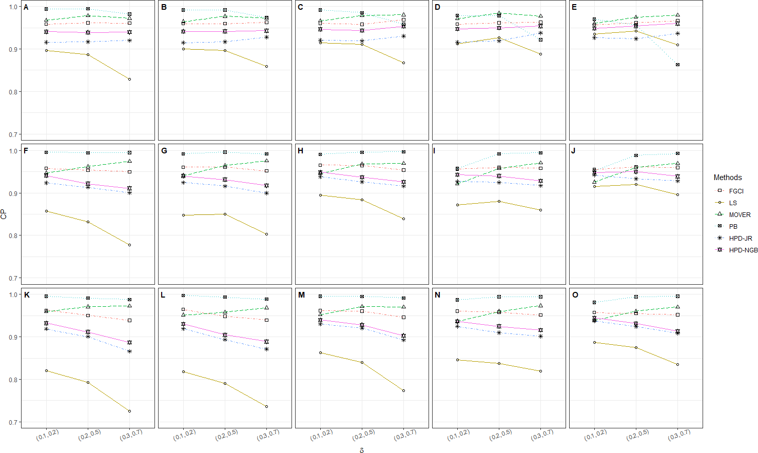
Figure 1: CP performances of 95%CIs for ϑ: 2 sample cases in the following cases (sample sizes, variances): (A) (302, 1, 2), (B) (30, 30, 2, 4), (C) (30, 30, 3, 5), (D) (30, 50, 1, 2), (E) (30, 50, 2, 4), (F) (30, 50, 3, 5), (G) (502, 1, 2), (H) (502, 2, 4), (I) (502, 3, 5), (J) (50, 100, 1, 2), (K) (50, 100, 2, 4), (L) (50, 100, 3, 5), (M) (1002, 1, 2), (N) (1002, 2, 4), (O) (1002, 3, 5).
Algorithm 6: Comparison of CPs and ALs for all CIs
-
For g = 1 to M. Generate .
-
Compute the unbiased estimates , and .
-
Compute the 95%CIs for ϑ based on FGCI, LS, MOVER, PB and the HPDs via Algorithm 1, 2, 3, 4 and 5, respectively.
-
Let Ag = 1 if ϑ falls within the intervals of FGCI, LS, MOVER, PB or the HPDs, else Ag = 0.
-
The CP and AL for each method are obtained by and AL = (U − L)∕M, respectively, where U and L are the upper and lower confidence limits, respectively. (end g loop)
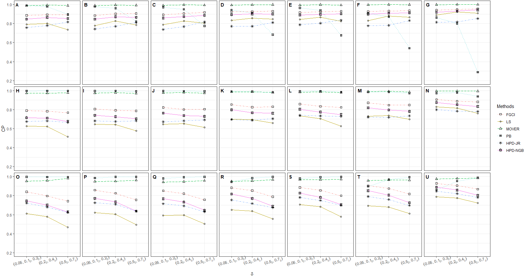
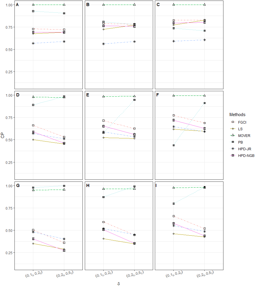
The numerical results for the CI performances are presented in terms of CP and AL for various sample cases. For k = 2 (Table 2 and Fig. 1), FGCI performed well for small-to-moderate sample sizes, as well as for large and a moderate-to-large sample size. HPD-NGB attained stable and the best CP and AL values for small and a moderate-to-large sample size. MOVER and PB attained correct CPs but wider ALs than the other methods whereas LS and HPD-JR had lower CPs and narrower ALs. For k = 5 (Table 3 and Fig. 2), there were only two methods producing better CPs than the other methods in the various situations: MOVER (small δi and ) and PB (large δi and ). Moreover, the results were similar for k = 10 (Table 4 and Fig. 3).
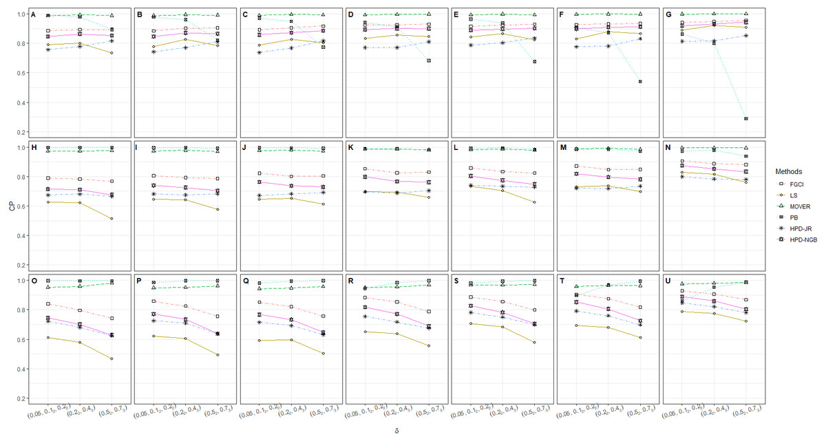
Figure 2: CP performances of 95%CIs for ϑ: 5 sample cases in the following cases (sample sizes, variances): (A) (305, 12, 23), (B) (305, 22, 33), (C) (305, 32, 53), (D) (302, 503, 12, 23), (E) (302, 503, 22, 33), (F) (302, 503, 32, 53), (G) (302, 503, 100, 12, 23), (H) (302, 503, 100, 22, 33), (I) (302, 503, 100, 32, 53), (J) (30, 502, 1002, 12, 23), (K) (30, 502, 1002, 12, 23), (L) (30, 502, 1002, 12, 23), (M) (505, 12, 23), (N) (505, 22, 33), (O) (505, 32, 53), (P) (502, 1003, 12, 23), (Q) (502, 1003, 22, 33), (R) (502, 1003, 32, 53), (S) (1005, 12, 23), (T) (1005, 22, 33), (U) (1005, 32, 53).
| Scenarios | CP | AL | ||||||||||
|---|---|---|---|---|---|---|---|---|---|---|---|---|
| FG | LS | MO | PB | HJ | HN | FG | LS | MO | PB | HJ | HN | |
| k = 5 | ||||||||||||
| 46 | 0.885 | 0.790 | 0.988 | 0.989 | 0.757 | 0.846 | 0.963 | 0.819 | 1.794 | 1.532 | 0.848 | 0.956 |
| 47 | 0.789 | 0.627 | 0.973 | 0.996 | 0.674 | 0.715 | 2.240 | 1.908 | 4.982 | 3.897 | 1.991 | 2.176 |
| 48 | 0.840 | 0.613 | 0.953 | 0.997 | 0.723 | 0.746 | 5.325 | 4.529 | 13.769 | 12.250 | 4.744 | 4.870 |
| 49 | 0.894 | 0.800 | 0.993 | 0.978 | 0.779 | 0.864 | 0.900 | 0.765 | 1.825 | 1.439 | 0.773 | 0.905 |
| 50 | 0.783 | 0.623 | 0.972 | 0.998 | 0.680 | 0.711 | 2.008 | 1.711 | 5.203 | 3.608 | 1.750 | 1.955 |
| 51 | 0.797 | 0.580 | 0.959 | 0.996 | 0.680 | 0.701 | 4.700 | 4.066 | 16.626 | 11.353 | 4.118 | 4.287 |
| 52 | 0.893 | 0.735 | 0.989 | 0.896 | 0.816 | 0.853 | 0.753 | 0.589 | 2.849 | 1.433 | 0.636 | 0.764 |
| 53 | 0.768 | 0.517 | 0.977 | 0.997 | 0.666 | 0.676 | 1.474 | 1.168 | 19.967 | 3.364 | 1.282 | 1.406 |
| 54 | 0.742 | 0.467 | 0.983 | 0.996 | 0.624 | 0.629 | 3.250 | 2.654 | 1.5e4 | 11.238 | 2.817 | 2.855 |
| 55 | 0.884 | 0.779 | 0.988 | 0.979 | 0.743 | 0.846 | 0.940 | 0.777 | 1.739 | 1.434 | 0.857 | 0.930 |
| 56 | 0.806 | 0.645 | 0.973 | 0.995 | 0.681 | 0.740 | 2.204 | 1.822 | 4.586 | 3.561 | 2.045 | 2.141 |
| 57 | 0.858 | 0.622 | 0.949 | 0.986 | 0.725 | 0.771 | 5.620 | 4.542 | 12.575 | 12.073 | 5.122 | 5.162 |
| 58 | 0.901 | 0.827 | 0.995 | 0.962 | 0.770 | 0.870 | 0.845 | 0.728 | 1.699 | 1.326 | 0.771 | 0.841 |
| 59 | 0.793 | 0.644 | 0.978 | 0.997 | 0.675 | 0.726 | 1.904 | 1.629 | 4.351 | 3.262 | 1.750 | 1.850 |
| 60 | 0.825 | 0.605 | 0.952 | 0.997 | 0.710 | 0.734 | 4.753 | 4.058 | 12.745 | 10.793 | 4.373 | 4.353 |
| 61 | 0.905 | 0.785 | 0.992 | 0.822 | 0.809 | 0.865 | 0.685 | 0.564 | 1.632 | 1.219 | 0.620 | 0.686 |
| 62 | 0.786 | 0.578 | 0.969 | 0.993 | 0.683 | 0.704 | 1.368 | 1.142 | 4.477 | 2.775 | 1.260 | 1.309 |
| 63 | 0.755 | 0.496 | 0.963 | 0.998 | 0.639 | 0.637 | 3.177 | 2.714 | 18.995 | 8.911 | 2.884 | 2.822 |
| 64 | 0.892 | 0.787 | 0.991 | 0.970 | 0.737 | 0.858 | 0.928 | 0.751 | 1.740 | 1.364 | 0.872 | 0.919 |
| 65 | 0.822 | 0.647 | 0.975 | 0.996 | 0.673 | 0.763 | 2.168 | 1.738 | 4.371 | 3.326 | 2.047 | 2.114 |
| 66 | 0.852 | 0.593 | 0.943 | 0.981 | 0.715 | 0.767 | 5.710 | 4.413 | 12.195 | 11.422 | 5.267 | 5.278 |
| 67 | 0.905 | 0.827 | 0.996 | 0.949 | 0.768 | 0.873 | 0.816 | 0.697 | 1.637 | 1.256 | 0.770 | 0.811 |
| 68 | 0.801 | 0.654 | 0.979 | 0.995 | 0.683 | 0.737 | 1.839 | 1.549 | 4.069 | 3.016 | 1.753 | 1.797 |
| 69 | 0.821 | 0.595 | 0.947 | 0.994 | 0.693 | 0.733 | 4.806 | 3.976 | 12.174 | 10.326 | 4.431 | 4.432 |
| 70 | 0.917 | 0.803 | 0.994 | 0.775 | 0.817 | 0.886 | 0.650 | 0.539 | 1.499 | 1.133 | 0.616 | 0.650 |
| 71 | 0.804 | 0.612 | 0.973 | 0.992 | 0.692 | 0.730 | 1.310 | 1.094 | 3.962 | 2.543 | 1.236 | 1.262 |
| 72 | 0.756 | 0.502 | 0.958 | 0.997 | 0.631 | 0.646 | 3.158 | 2.695 | 16.604 | 8.356 | 2.888 | 2.835 |
| 73 | 0.924 | 0.832 | 0.994 | 0.942 | 0.772 | 0.893 | 0.822 | 0.673 | 1.505 | 1.186 | 0.856 | 0.808 |
| 74 | 0.853 | 0.699 | 0.985 | 0.990 | 0.696 | 0.798 | 1.971 | 1.589 | 3.823 | 2.899 | 2.000 | 1.923 |
| 75 | 0.883 | 0.652 | 0.952 | 0.945 | 0.755 | 0.817 | 5.330 | 4.072 | 9.997 | 9.911 | 5.224 | 4.974 |
| 76 | 0.924 | 0.857 | 0.997 | 0.913 | 0.771 | 0.901 | 0.723 | 0.626 | 1.418 | 1.088 | 0.746 | 0.715 |
| 77 | 0.826 | 0.695 | 0.986 | 0.989 | 0.689 | 0.767 | 1.670 | 1.406 | 3.476 | 2.610 | 1.692 | 1.632 |
| 78 | 0.854 | 0.638 | 0.955 | 0.984 | 0.718 | 0.771 | 4.456 | 3.628 | 9.715 | 8.788 | 4.311 | 4.160 |
| 79 | 0.930 | 0.846 | 0.998 | 0.683 | 0.811 | 0.900 | 0.581 | 0.486 | 1.253 | 0.964 | 0.586 | 0.580 |
| 80 | 0.830 | 0.658 | 0.981 | 0.980 | 0.705 | 0.762 | 1.215 | 1.019 | 3.179 | 2.168 | 1.225 | 1.181 |
| 81 | 0.788 | 0.555 | 0.967 | 0.997 | 0.675 | 0.689 | 2.992 | 2.554 | 11.873 | 7.026 | 2.927 | 2.738 |
| 82 | 0.915 | 0.844 | 0.993 | 0.964 | 0.788 | 0.889 | 0.769 | 0.662 | 1.337 | 1.158 | 0.692 | 0.753 |
| 83 | 0.858 | 0.735 | 0.982 | 0.993 | 0.741 | 0.804 | 1.882 | 1.599 | 3.605 | 2.920 | 1.698 | 1.825 |
| 84 | 0.886 | 0.705 | 0.969 | 0.981 | 0.782 | 0.827 | 4.650 | 3.895 | 8.767 | 9.068 | 4.208 | 4.335 |
| 85 | 0.925 | 0.865 | 0.998 | 0.939 | 0.803 | 0.897 | 0.707 | 0.618 | 1.315 | 1.068 | 0.618 | 0.700 |
| 86 | 0.834 | 0.705 | 0.987 | 0.994 | 0.735 | 0.775 | 1.683 | 1.439 | 3.493 | 2.683 | 1.482 | 1.642 |
| 87 | 0.855 | 0.684 | 0.968 | 0.994 | 0.751 | 0.783 | 4.027 | 3.489 | 8.924 | 8.068 | 3.613 | 3.766 |
| 88 | 0.929 | 0.824 | 0.994 | 0.677 | 0.835 | 0.903 | 0.611 | 0.495 | 1.322 | 0.993 | 0.515 | 0.616 |
| 89 | 0.823 | 0.627 | 0.981 | 0.985 | 0.729 | 0.749 | 1.284 | 1.045 | 3.692 | 2.296 | 1.121 | 1.250 |
| 90 | 0.799 | 0.578 | 0.972 | 0.997 | 0.699 | 0.705 | 2.875 | 2.453 | 13.603 | 6.644 | 2.519 | 2.641 |
| 91 | 0.927 | 0.831 | 0.997 | 0.906 | 0.777 | 0.898 | 0.753 | 0.614 | 1.389 | 1.064 | 0.703 | 0.735 |
| 92 | 0.871 | 0.731 | 0.988 | 0.986 | 0.720 | 0.820 | 1.821 | 1.466 | 3.459 | 2.601 | 1.721 | 1.769 |
| 93 | 0.905 | 0.693 | 0.957 | 0.897 | 0.791 | 0.852 | 5.015 | 3.768 | 8.461 | 8.829 | 4.621 | 4.690 |
| 94 | 0.931 | 0.879 | 0.999 | 0.873 | 0.781 | 0.909 | 0.651 | 0.571 | 1.279 | 0.972 | 0.608 | 0.639 |
| 95 | 0.847 | 0.738 | 0.991 | 0.986 | 0.719 | 0.797 | 1.541 | 1.313 | 3.117 | 2.351 | 1.447 | 1.499 |
| 96 | 0.875 | 0.679 | 0.966 | 0.969 | 0.760 | 0.806 | 4.125 | 3.374 | 8.002 | 7.707 | 3.808 | 3.865 |
| 97 | 0.935 | 0.866 | 0.998 | 0.541 | 0.832 | 0.911 | 0.529 | 0.450 | 1.097 | 0.856 | 0.493 | 0.523 |
| 98 | 0.848 | 0.697 | 0.986 | 0.971 | 0.735 | 0.782 | 1.126 | 0.956 | 2.572 | 1.916 | 1.060 | 1.091 |
| 99 | 0.817 | 0.613 | 0.963 | 0.994 | 0.698 | 0.725 | 2.784 | 2.418 | 7.510 | 6.042 | 2.565 | 2.571 |
| 100 | 0.941 | 0.888 | 0.998 | 0.863 | 0.813 | 0.920 | 0.557 | 0.484 | 0.954 | 0.806 | 0.510 | 0.536 |
| 101 | 0.906 | 0.827 | 0.995 | 0.973 | 0.799 | 0.875 | 1.413 | 1.201 | 2.515 | 2.029 | 1.288 | 1.361 |
| 102 | 0.929 | 0.790 | 0.975 | 0.861 | 0.845 | 0.889 | 3.639 | 2.946 | 5.529 | 6.174 | 3.365 | 3.428 |
| 103 | 0.948 | 0.923 | 1.000 | 0.801 | 0.816 | 0.931 | 0.501 | 0.456 | 0.909 | 0.741 | 0.452 | 0.487 |
| 104 | 0.888 | 0.816 | 0.996 | 0.978 | 0.784 | 0.853 | 1.253 | 1.095 | 2.373 | 1.852 | 1.121 | 1.216 |
| 105 | 0.905 | 0.775 | 0.981 | 0.953 | 0.822 | 0.859 | 3.147 | 2.678 | 5.326 | 5.441 | 2.893 | 2.975 |
| 106 | 0.955 | 0.907 | 0.999 | 0.289 | 0.852 | 0.943 | 0.438 | 0.372 | 0.838 | 0.668 | 0.373 | 0.433 |
| 107 | 0.881 | 0.761 | 0.994 | 0.939 | 0.781 | 0.833 | 0.992 | 0.823 | 2.044 | 1.536 | 0.863 | 0.972 |
| 108 | 0.868 | 0.722 | 0.984 | 0.987 | 0.781 | 0.805 | 2.331 | 2.005 | 5.072 | 4.308 | 2.088 | 2.208 |
Notes:
- FG
-
fiducial generalized confidence interval
- MO
-
method of variance estimates
- HJ
-
HPD-based Jeffreys’ rule prior
- HPD-JR
-
HN, HPD-based normal-gamma-beta prior
Bold denoted as the best-performing method each case.
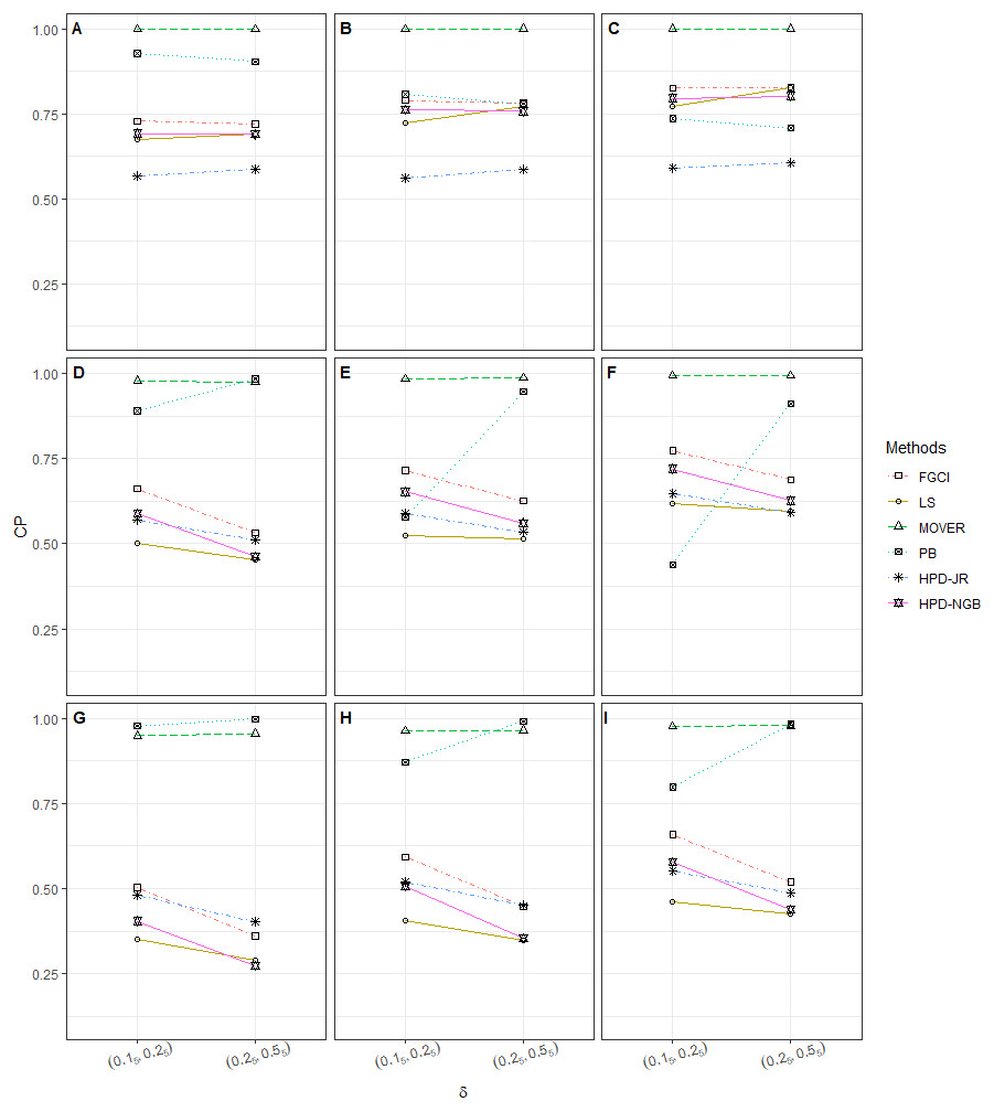
Figure 3: CP performances of 95%CIs for ϑ: 10 sample cases in the following cases (sample sizes, variances): (A) (305, 505, 12, 25), (B) (305, 505, 25, 45), (C) (305, 505, 35, 55), (D) (303, 503, 1004, 12, 25), (E) (303, 503, 1004, 25, 45), (F) (303, 503, 1004, 35, 55), (G) (505, 1005, 15, 25), (H) (505, 1005, 25, 45), (I) (505, 1005, 32, 53).
| CP | AL | |||||||||||
|---|---|---|---|---|---|---|---|---|---|---|---|---|
| Scenarios | FG | LS | MO | PB | HJ | HN | FG | LS | MO | PB | HJ | HN |
| k = 10 | ||||||||||||
| 109 | 0.728 | 0.675 | 0.998 | 0.927 | 0.566 | 0.692 | 0.612 | 0.501 | 1.554 | 0.932 | 0.545 | 0.623 |
| 110 | 0.661 | 0.500 | 0.979 | 0.891 | 0.570 | 0.588 | 1.644 | 1.291 | 3.867 | 3.278 | 1.500 | 1.637 |
| 111 | 0.504 | 0.352 | 0.950 | 0.978 | 0.481 | 0.404 | 3.159 | 2.561 | 8.645 | 7.286 | 2.996 | 3.076 |
| 112 | 0.720 | 0.692 | 0.999 | 0.904 | 0.587 | 0.690 | 0.557 | 0.459 | 1.519 | 0.832 | 0.483 | 0.574 |
| 113 | 0.532 | 0.452 | 0.976 | 0.985 | 0.512 | 0.462 | 1.393 | 1.159 | 3.853 | 2.682 | 1.260 | 1.404 |
| 114 | 0.361 | 0.290 | 0.955 | 0.998 | 0.403 | 0.274 | 2.556 | 2.218 | 8.570 | 5.943 | 2.411 | 2.505 |
| 115 | 0.789 | 0.723 | 0.999 | 0.808 | 0.561 | 0.762 | 0.554 | 0.440 | 1.416 | 0.789 | 0.546 | 0.560 |
| 116 | 0.716 | 0.524 | 0.985 | 0.578 | 0.590 | 0.653 | 1.635 | 1.180 | 3.478 | 2.915 | 1.559 | 1.624 |
| 117 | 0.593 | 0.406 | 0.964 | 0.872 | 0.519 | 0.507 | 3.289 | 2.406 | 7.754 | 6.380 | 3.189 | 3.214 |
| 118 | 0.782 | 0.773 | 1.000 | 0.780 | 0.586 | 0.758 | 0.477 | 0.404 | 1.317 | 0.696 | 0.474 | 0.483 |
| 119 | 0.626 | 0.514 | 0.988 | 0.947 | 0.535 | 0.561 | 1.337 | 1.076 | 3.348 | 2.360 | 1.284 | 1.341 |
| 120 | 0.447 | 0.347 | 0.965 | 0.992 | 0.450 | 0.355 | 2.570 | 2.108 | 7.290 | 5.180 | 2.506 | 2.531 |
| 121 | 0.826 | 0.773 | 1.000 | 0.736 | 0.592 | 0.796 | 0.488 | 0.399 | 1.266 | 0.695 | 0.444 | 0.486 |
| 122 | 0.774 | 0.620 | 0.994 | 0.438 | 0.647 | 0.720 | 1.460 | 1.086 | 3.072 | 2.512 | 1.328 | 1.438 |
| 123 | 0.659 | 0.460 | 0.977 | 0.798 | 0.553 | 0.577 | 3.002 | 2.236 | 6.597 | 5.502 | 2.775 | 2.921 |
| 124 | 0.828 | 0.826 | 1.000 | 0.708 | 0.606 | 0.802 | 0.426 | 0.368 | 1.187 | 0.615 | 0.387 | 0.427 |
| 125 | 0.688 | 0.595 | 0.995 | 0.912 | 0.591 | 0.627 | 1.205 | 0.992 | 2.912 | 2.039 | 1.094 | 1.197 |
| 126 | 0.520 | 0.426 | 0.979 | 0.984 | 0.486 | 0.439 | 2.390 | 1.989 | 6.222 | 4.479 | 2.224 | 2.344 |
Notes:
- FG
-
fiducial generalized confidence interval
- MO
-
method of variance estimates recovery
- HJ
-
HPD-based Jeffreys’ rule prior
- HPD-JR
-
HN, HPD-based normal-gamma-beta prior
Bold denoted as the best-performing method each case.
As previously mentioned, our findings show that FGCI works well for small sample case because the FGPQ of might contain some weak points that affect the FGPQ of μi as the sample case increases. For large sample sizes, MOVER was the best method for small σ2, which is possibly caused by the CI for . Meanwhile, the next best one was PB, which has the strong point of using a resampling technique to collect information about several populations even when the variance σ2 is large.
| Northern | Northeastern | Central | Eastern | Southern | |||||||||||
|---|---|---|---|---|---|---|---|---|---|---|---|---|---|---|---|
| 3 | 0 | 3 | 0 | 0 | 49.5 | 0 | 0 | 0 | 2.9 | 3.2 | 0 | 4.1 | 0 | 0 | 2.7 |
| 2.6 | 5 | 0 | 40 | 1.5 | 10.5 | 0 | 0 | 0 | 0.2 | 0 | 3.2 | 0 | 0 | 0 | 0 |
| 1 | 23.8 | 0 | 3.5 | 18.5 | 60.4 | 4 | 0 | 11 | 0.3 | 0 | 10.4 | 11.5 | 3.5 | 0 | 0 |
| 3.6 | 16 | 0 | 0 | 42 | 12.7 | 0 | 0 | 0 | 2.5 | 4.7 | 1.1 | 2.5 | 13.6 | 0 | 0 |
| 0 | 11.5 | 0 | 12 | 9.1 | 6.8 | 0 | 20.3 | 0 | 0.4 | 19.3 | 0.2 | 9.7 | 0 | 0.2 | 0 |
| 13.2 | 1.2 | 0 | 15 | 6 | 69.3 | 0 | 0 | 0 | 0.4 | 3.1 | 4.3 | 10.4 | 0 | 0 | 0 |
| 22.4 | 10.3 | 0 | 0 | 7.5 | 36.5 | 0 | 2.4 | 0.3 | 1.1 | 2.9 | 0 | 9.6 | 0 | 0 | 0 |
| 1.4 | 1.7 | 0 | 1.5 | 0 | 8.6 | 0 | 0 | 1 | 0 | 5.7 | 0 19 | 0 | 0 | 0 | |
| 18.3 | 5.5 | 0 | 0.7 | 6.3 | 0 | 0 | 0 | 0 | 1.3 | 0.9 | 0 | 8.3 | 0 | 0 | 0 |
| 0 | 7.3 | 0 | 0 | 0 | 0 | 0 | 0 | 0 | 0.1 | 0 | 0 | 0 | 4.8 | 0 | 6.2 |
| 15.5 | 24.3 | 1.7 | 3 | 0.4 | 0 | 0 | 0 | 0 | 2.9 | 0 | 0.2 | 0 | 0 | 0 | 0 |
| 0 | 27.2 | 2.3 | 0 | 0 | 3.8 | 0 | 0 | 0 | 0 | 2.6 | 0.1 | 0 | 0 | 0 | 0 |
| 0 | 12.6 | 0.5 | 0 | 0 | 0 | 0 | 3.2 | 0 | 1 | 17 | 62.8 | 0 | 0 | 0 | 6.1 |
| 0 | 22.7 | 3.9 | 0 | 0 | 0 | 0 | 0 | 0 | 4.7 | 0 | 36.7 | 17.8 | 0 | 0 | 0 |
| 9.8 | 0 | 6.9 | 29.4 | 1.8 | 0 | 0 | 0 | 0 | 0.5 | 3.5 | 15.6 | 12.3 | 0 | 0 | 0 |
| 24.3 | 2.6 | 2.2 | 48 | 0 | 0 | 0 | 0 | 0 | 5 | 0 | 50 | 2.5 | 0 | 0 | 0 |
| 24.6 | 0 | 3.2 | 0 | 0 | 0 | 6 | 0 | 0 | 2.5 | 0 | 35.5 | 0 | 0 | 0 | 0.3 |
| 8.8 | 3.2 | 5.3 | 70.8 | 14.3 | 0 | 0 | 0 | 0 | 0 | 0 | 35 | 0.9 | 0 | 0 | 0 |
| 0 | 2.6 | 11 | 3.5 | 0 | 0 | 0 | 0 | 0 | 0 | 5.1 | 5.9 | 0 | 0 | 0 | 0 |
| 19.8 | 2 | 0.6 | 14.2 | 0 | 0 | 0 | 4.8 | 0 | 0 | 60.4 | 0 | 2.6 | 0 | 0 | 0 |
| 5 | 8 | 0 | 7 | 0 | 0 | 2.3 | 0 | 0 | 0 | 6.9 | 0 | 0 | 0 | 0 | 0 |
| 12.3 | 1.9 | 1 | 0 | 0 | 21.5 | 0 | 0 | 0 | 6.6 | 3 | 3 | 0 | 0 | 0 | 0 |
| 8.1 | 0.8 | 2.4 | 0 | 0 | 2.5 | 1 | 0 | 0 | 0 | 15.1 | 60.4 | 2 | 0 | 0 | 0 |
| 4.8 | 2.2 | 13.2 | 0 | 0 | 0 | 0 | 0 | 0 | 9.5 | 6 | 60 | 0 | 0 | 0 | 0 |
| 5.8 | 6.5 | 0.4 | 0 | 0 | 13 | 0 | 0 | 5.1 | 13.4 | 76 | 0 | 0 | 0 | 0 | |
| 17 | 0 | 0 | 10.8 | 0 | 26.2 | 0 | 0 | 12.5 | 6.2 | 79.7 | 0 | 0 | 0 | 0 | |
| 25.1 | 2.2 | 1.3 | 0 | 10.1 | 2.2 | 4.6 | 5.4 | 0 | 65.7 | 3.5 | 0 | 0 | |||
| 8.3 | 0 | 10 | 6.3 | 0 | 3 | 0 | 0 | 0 | 108 | 0 | 0 | 36.1 | |||
| 22.9 | 4.3 | 2.5 | 0 | 4.8 | 10.5 | 10 | 0 | 3.2 | 10.5 | 0 | 0 | 41.8 | |||
| 26.9 | 0.2 | 4.6 | 4 | 0 | 0 | 0 | 12 | 0 | 0 | 0 | 30 | ||||
| 0 | 0 | 0 | 19.3 | 0 | 0 | 9.5 | 0 | 2.2 | 0 | 0 | 0 | ||||
Notes:
Source: Thai Meteorological Department: https://www.tmd.go.th/services/weekly report.php.
| Northern | Northeastern | Central | Eastern | Southern | |||||||||||
|---|---|---|---|---|---|---|---|---|---|---|---|---|---|---|---|
| 9.5 | 0 | 25.3 | 20 | 6.6 | 8.4 | 0 | 67 | 0 | 39.6 | 0 | 0 | 27.9 | 4.1 | 0.4 | 114.6 |
| 4.9 | 10 | 25.5 | 14.5 | 16.9 | 0.8 | 2.9 | 65.4 | 0 | 25 | 0 | 0 | 0 | 9 | 3.8 | 0 |
| 0 | 21.6 | 24 | 3 | 10 | 20.2 | 0 | 21 | 0 | 0 | 0 | 26.5 | 3.4 | 27.3 | 0.6 | 0 |
| 4.7 | 15 | 8 | 28 | 48.2 | 0 | 14.3 | 6.4 | 7.2 | 0 | 0 | 36.4 | 0 | 6.5 | 0 | 0 |
| 0 | 15.5 | 0 | 27 | 6.5 | 0.5 | 0 | 0 | 3.5 | 29.7 | 0.1 | 0 | 0.8 | 3.5 | 10.8 | 0 |
| 63.2 | 14 | 20 | 50 | 4.8 | 5.3 | 6 | 52 | 0 | 0 | 0.3 | 4.5 | 37.9 | 0 | 5 | 18.2 |
| 9.6 | 8.5 | 0 | 24 | 25 | 16.7 | 0 | 45 | 40.5 | 3.1 | 0.5 | 0 | 32.4 | 0 | 12.2 | 40.4 |
| 10.7 | 11.5 | 0 | 30 | 0 | 45.2 | 28 | 41.4 | 25.8 | 8.2 | 31.5 | 0.5 | 33.8 | 0 | 3.6 | 0 |
| 13 | 17.4 | 0 | 22 | 0 | 0 | 0 | 14.3 | 30.4 | 3.2 | 8.2 | 0.7 | 15.8 | 0 | 0 | 0 |
| 0 | 15.6 | 0 | 16 | 3.2 | 0.6 | 0 | 45 | 0 | 7.1 | 0 | 12.3 | 0 | 3.6 | 8.8 | 10.8 |
| 0 | 31.6 | 33.8 | 0 | 44 | 0 | 0 | 27 | 0 | 0 | 0 | 0.5 | 0 | 3 | 0 | 0 |
| 0 | 20.6 | 33.7 | 0 | 0 | 3.1 | 27.6 | 0.2 | 0 | 3.2 | 0 | 1.9 | 0 | 1 | 0 | 0 |
| 0 | 31.1 | 15.1 | 0 | 9.3 | 33.3 | 33 | 30 | 0 | 4.2 | 0 | 66.4 | 0 | 3.7 | 6.2 | 35 |
| 0 | 16.3 | 18.5 | 0 | 0 | 6 | 0 | 0 | 0 | 5.7 | 0 | 93.6 | 11.5 | 15.6 | 0 | 0 |
| 2.8 | 0 | 44.8 | 39.7 | 20 | 0 | 0 | 0 | 8.3 | 30 | 0 | 68.7 | 1.7 | 11.2 | 3.8 | 33.5 |
| 11.3 | 33.1 | 37.5 | 9.3 | 0 | 13.2 | 0 | 0 | 0 | 4 | 0 | 40 | 1.2 | 24 | 0 | 57 |
| 0.6 | 29.2 | 0 | 0 | 4.8 | 0 | 0 | 0 | 0 | 0 | 0 | 65 | 21.2 | 0 | 0 | 10.5 |
| 36.1 | 11.2 | 47 | 2.1 | 0 | 21 | 0 | 0 | 0 | 0 | 0 | 63.7 | 0 | 0 | 0 | 0 |
| 0 | 14.4 | 20 | 0 | 0 | 0 | 0 | 1 | 36.1 | 0 | 0 | 9.2 | 30 | 10.2 | 0.2 | 0 |
| 2.6 | 60 | 30.8 | 46.7 | 0 | 8.4 | 15 | 0 | 0 | 0 | 1.2 | 0 | 5.1 | 0 | 0 | 0 |
| 5 | 42.3 | 30 | 10.5 | 0 | 0 | 0 | 0 | 12.5 | 0 | 0 | 0 | 2.5 | 0 | 0 | 30.8 |
| 13.4 | 9.5 | 1 | 0 | 56.5 | 0 | 0 | 2.5 | 0 | 14.7 | 0.1 | 11 | 2.4 | 0 | 0.4 | 10.7 |
| 12.3 | 34.5 | 1.2 | 41 | 39.2 | 0.5 | 0 | 0 | 0 | 0 | 1 | 69.6 | 5 | 0 | 0 | 0 |
| 25.8 | 36.5 | 56.3 | 10.3 | 0 | 4.5 | 25.7 | 9.5 | 0 | 0 | 3 | 89.6 | 1.7 | 0 | 0 | 15.9 |
| 30.2 | 9.7 | 0 | 1.2 | 6.4 | 16.2 | 41.4 | 0 | 0 | 0.5 | 160 | 0 | 0 | 2.2 | 0 | |
| 16.4 | 0 | 6 | 23.9 | 5.3 | 0 | 41.6 | 0 | 1.6 | 34.3 | 0 | 0 | 0 | |||
| 6 | 0 | 0 | 22.2 | 0 | 3.5 | 53.8 | 0 | 0 | 0 | 2.1 | 0 | 0.6 | |||
| 33.1 | 7.6 | 5.3 | 24.1 | 9.8 | 20 | 48.5 | 0 | 0 | 25 | 0 | 0 | 76.6 | |||
| 16.4 | 9.6 | 7.2 | 38 | 0 | 0 | 78.5 | 2.1 | 0 | 19.5 | 10.5 | 7 | 121.6 | |||
| 19.8 | 9.3 | 24.6 | 9 | 9.7 | 0 | 12.7 | 0 | 0 | 15.3 | 10.6 | 60 | ||||
| 0 | 0 | 30 | 9.2 | 4.5 | 1.2 | 80.9 | 0 | 0 | 0 | 3.6 | 0 | ||||
Notes:
Source: Thai Meteorological Department: https://www.tmd.go.th/services/weekly_report.php.
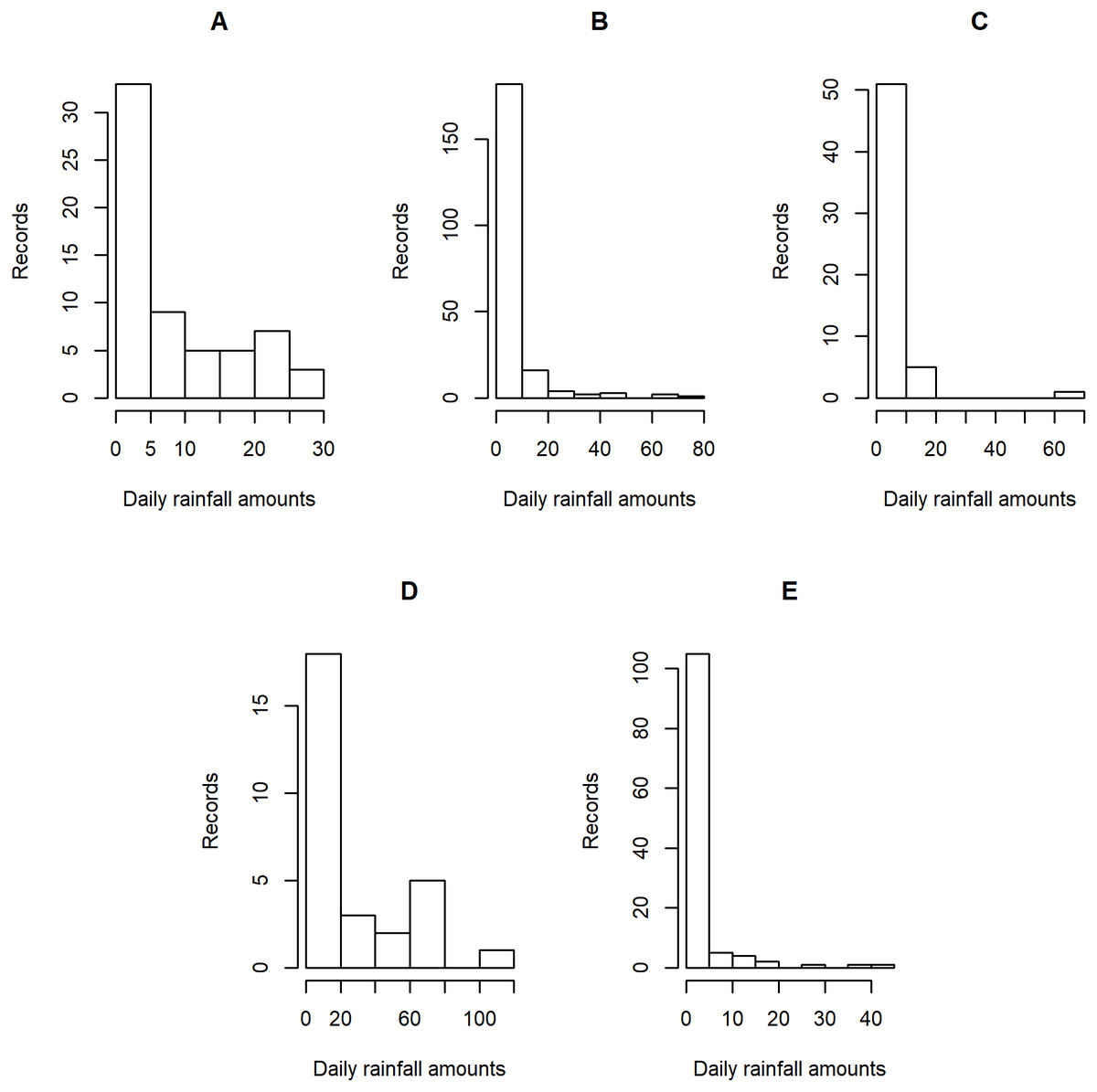
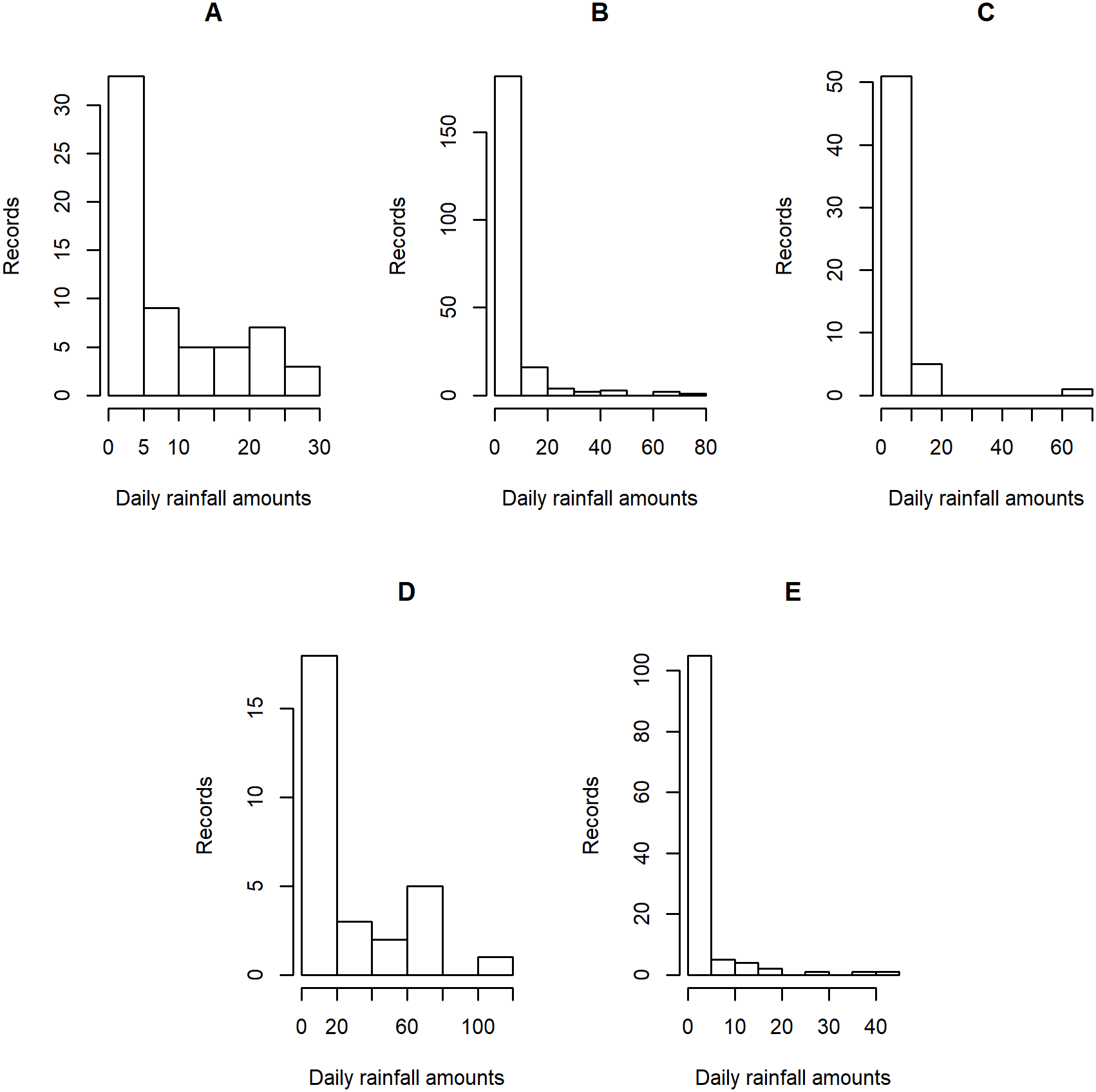
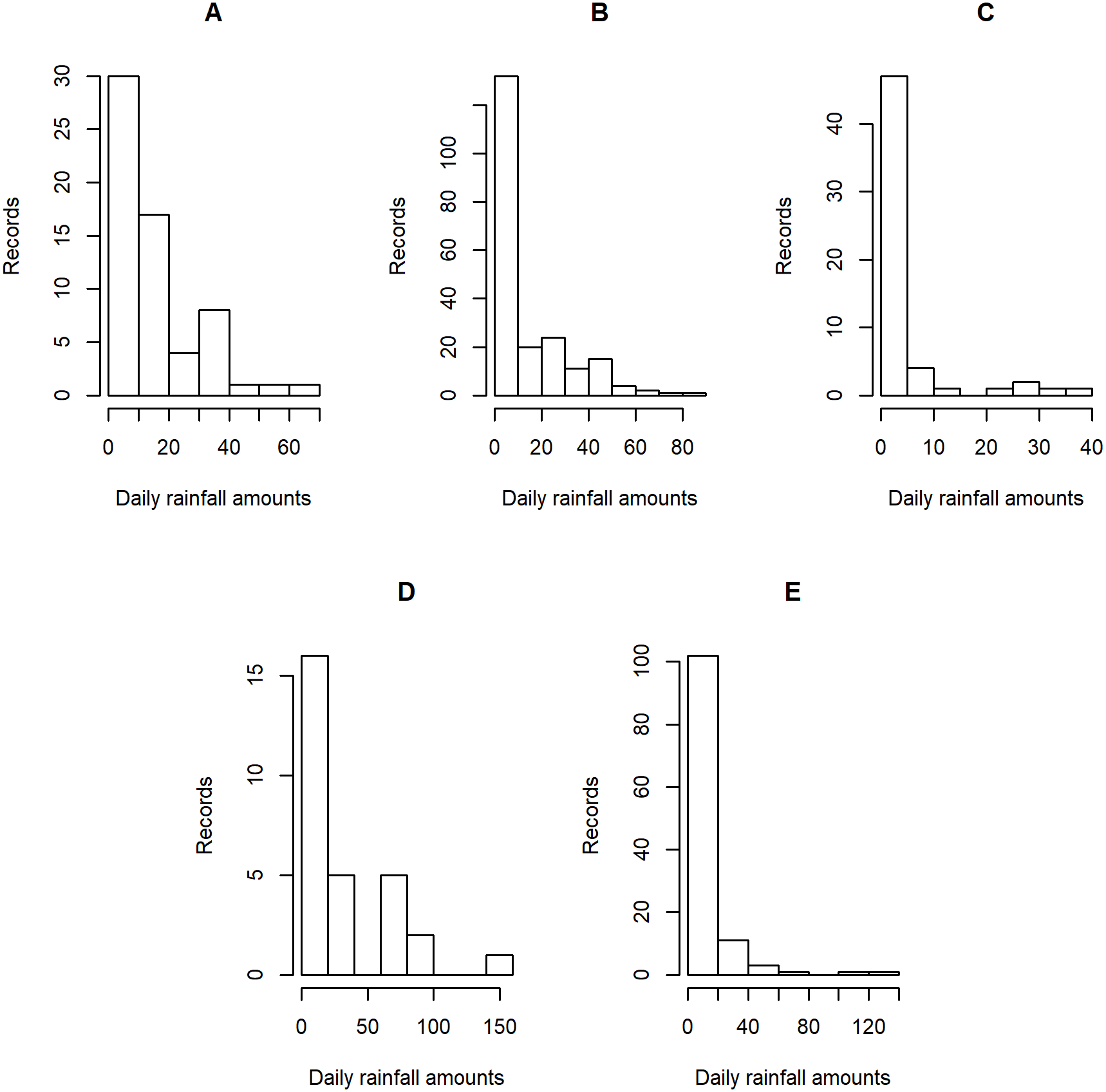
Figure 4: Histogram plots of daily rainfall data in five Thailand’s regions on August 5, 2019: (A) Northern (B) Northeastern (C) Central (D) Eastern (E) Southern.

Figure 5: Histogram plots of daily rainfall data in five Thailand’s regions on August 9, 2019: (A) Northern (B) Northeastern (C) Central (D) Eastern (E) Southern.
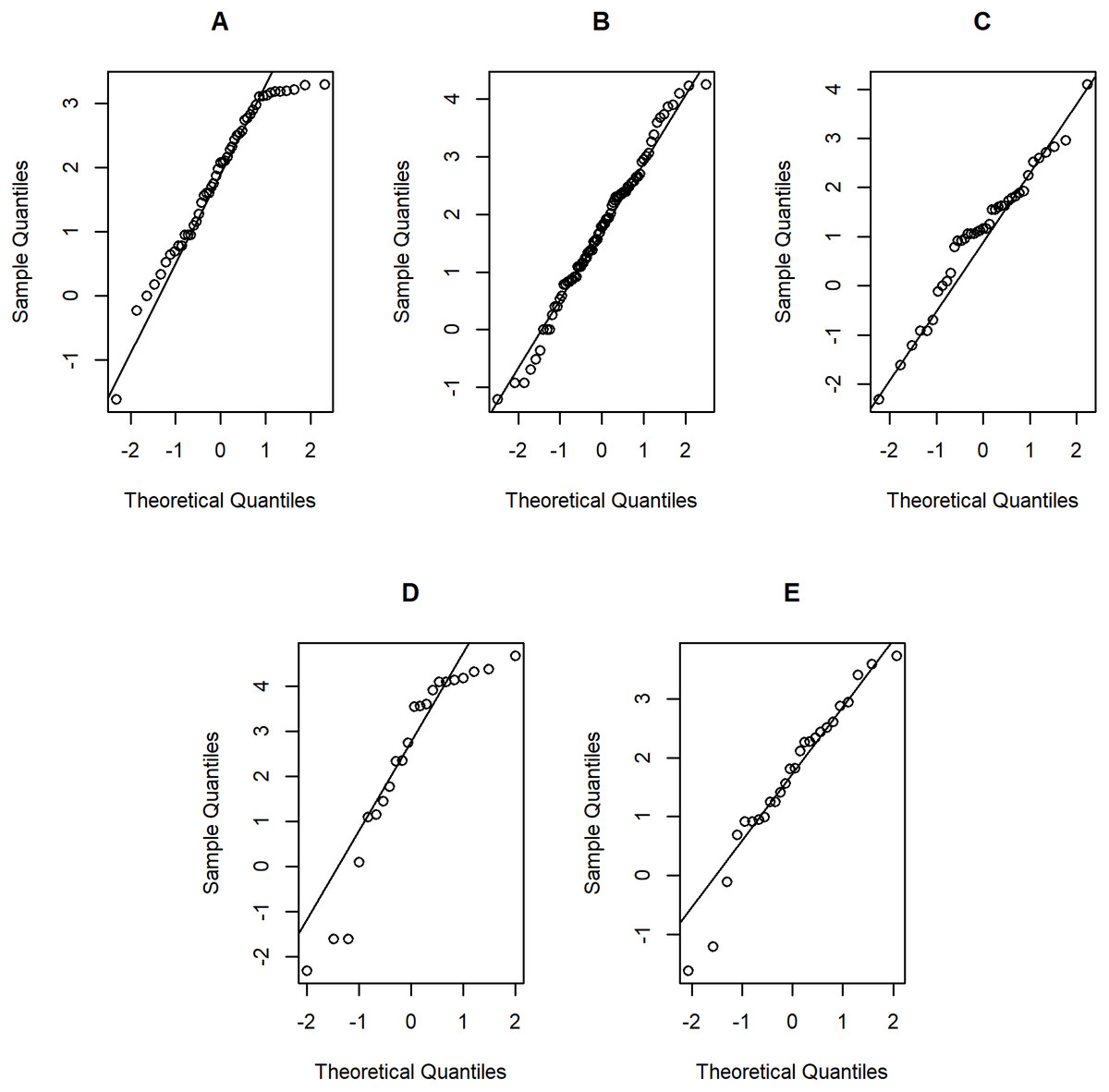
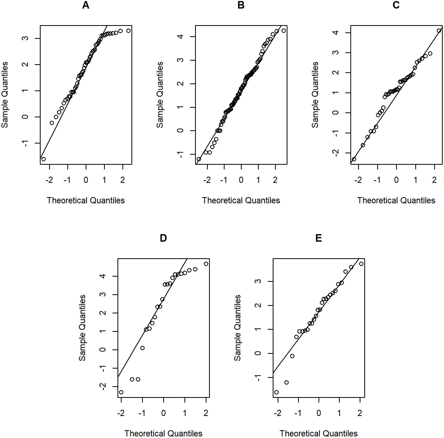
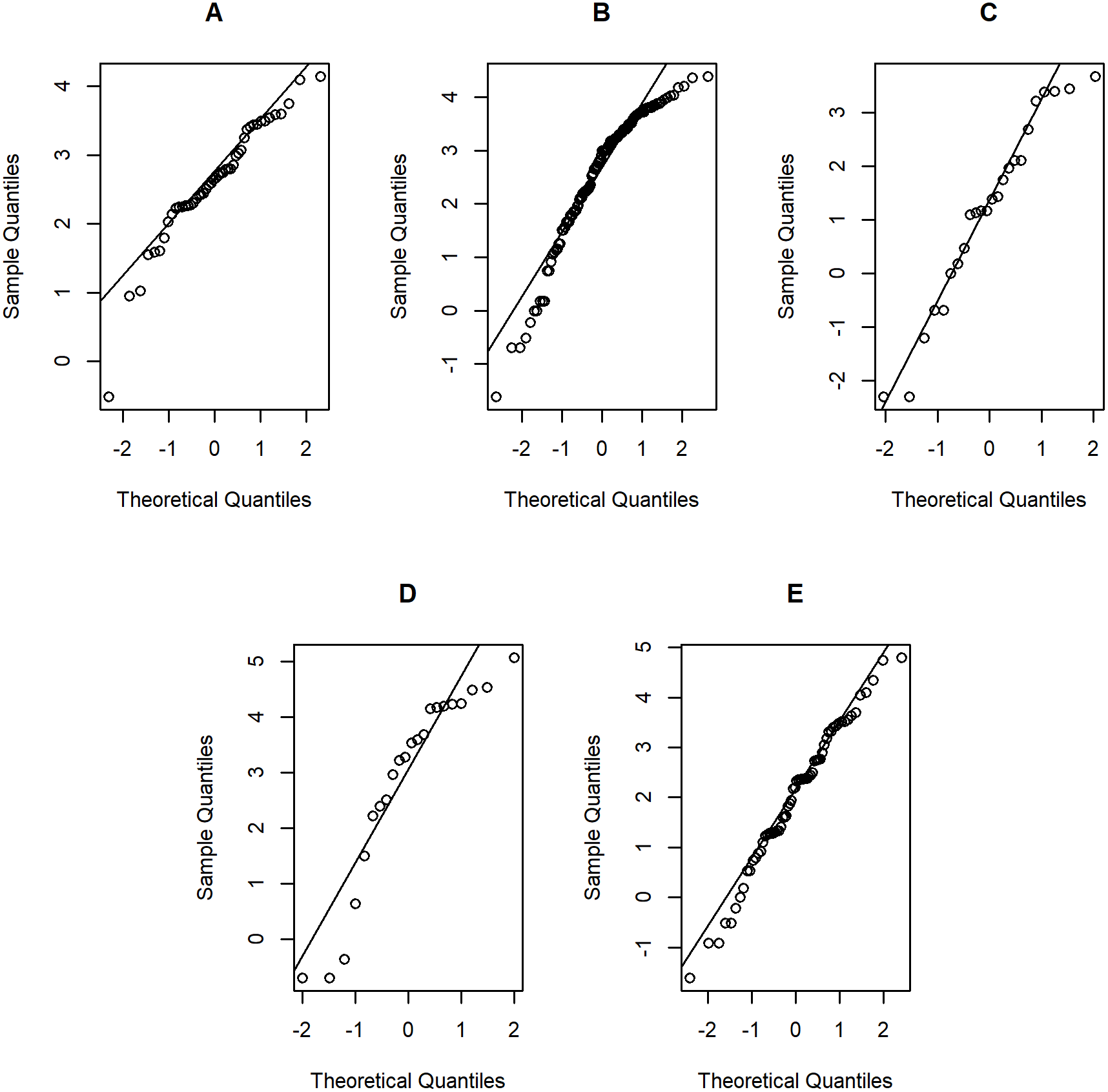
Figure 6: Normal Q-Q plots of log-positive daily rainfall data in five Thailand’s regions on August 5, 2019: (A) Northern (B) Northeastern (C) Central (D) Eastern (E) Southern.
An empirical application
Daily rainfall data obtained from the Thai Meteorological Department (TMD) were divided into the northern, northeastern, central, and eastern regions, while the southern region was a combination of the data from the southeastern and southwestern shores. Due to the differences in the climate patterns and meteorological conditions in the five regions, we focused was on estimating the daily rainfall data in these regions by treating them as separate sets of observations rather than using the average rainfall for the whole of Thailand by pooling them and treating them as a single population. The daily rainfall amounts were recorded on August 5 and 9, 2019, which is in the middle of the rainy season (mid-May to mid-October) when rice farming is conducted in Thailand. Entries with rainfall of less than 0.1 mm were considered as zero records.
Tables 5–6 contain the daily rainfall records for the five regions, while Figs. 4–5 show histogram plots of rainfall observations, and Figs. 6–7 exhibit normal Q-Q plots of the log-positive rainfall data on August 5 and 9, 2019, respectively. It can be seen that the data for all of the regions contained zero observations. After that, the fitted distribution of the positive observations was checked using the Akaike information criterion (AIC), as reported in Table 7. It can be concluded that the rainfall data in all of the regions on August 5 and 9, 2019 follow a delta-lognormal distribution. All data sets and R code are available in the Supplemental Information. The summary statistics are reported in Table 8. In the approximation of the daily rainfall amounts in the five regions, the estimated common means were 4.4506 and 13.2621 mm/day on August 5 and 9, 2019, respectively. The computed 95% CIs of the common rainfall mean are reported in Table 9. Under the rain criteria issued by the TMD (Department, 2018), it can be interpreted that the daily rainfall in Thailand on August 5, 2019, was light (0.1–10.0 mm), while it was moderate (10.1–35.0 mm) on August 9, 2019. These results confirm the simulation results for k = 5 in the previous section.
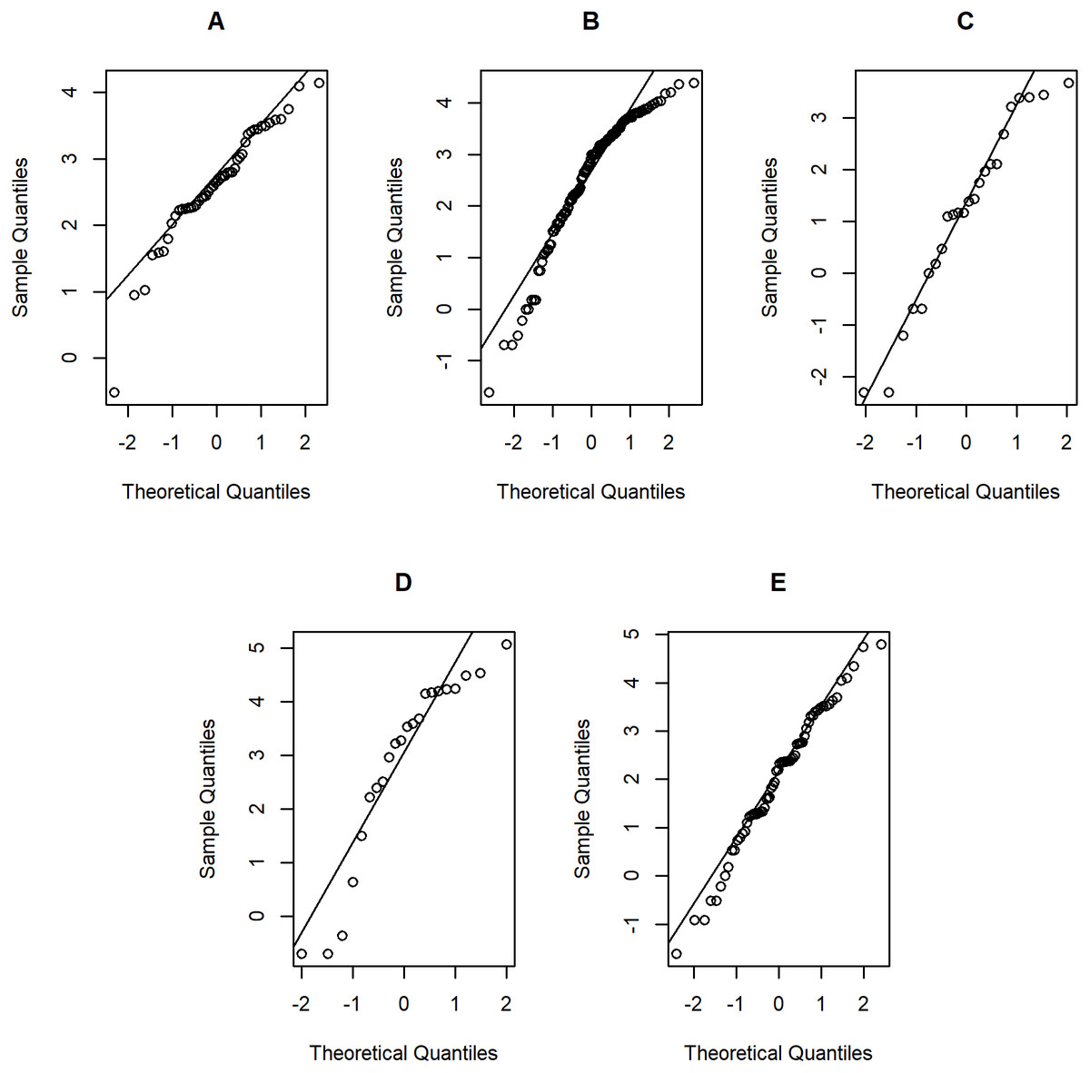
Figure 7: Normal Q-Q plots of log-positive daily rainfall data in five Thailand’s regions on August 9, 2019: (A) Northern (B) Northeastern (C) Central (D) Eastern (E) Southern.
| Regions | AIC | ||||
|---|---|---|---|---|---|
| Cauchy | Logistic | Lognormal | Normal | T-distribution | |
| On August 5, 2019 | |||||
| Northern | 373.1958 | 357.3122 | 336.8724 | 353.7757 | 354.3055 |
| Northeastern | 600.9473 | 642.1779 | 543.9619 | 667.2334 | 664.6152 |
| Central | 240.0227 | 266.4162 | 220.8503 | 293.9151 | 283.2302 |
| Eastern | 229.8995 | 220.2523 | 202.8394 | 218.7240 | 219.1471 |
| Southern | 194.9368 | 197.5586 | 178.5587 | 201.1654 | 200.1388 |
| On August 9, 2019 | |||||
| Northern | 389.6257 | 387.3072 | 375.7994 | 391.1802 | 390.2479 |
| Northeastern | 1123.7491 | 1080.8694 | 1052.8953 | 1080.1467 | 1079.9365 |
| Central | 178.8516 | 189.5353 | 155.0261 | 190.6855 | 190.5103 |
| Eastern | 233.5236 | 227.1725 | 215.9306 | 228.0501 | 227.4559 |
| Southern | 541.0477 | 569.2615 | 487.4667 | 592.2242 | 588.2377 |
| Regions | Estimated parameters | ||||
|---|---|---|---|---|---|
| ni | |||||
| August 5, 2020 | |||||
| Northern | 62 | 1.866 | 1.277 | 0.210 | 9.472 |
| Northeastern | 210 | 1.734 | 1.578 | 0.619 | 4.668 |
| Central | 57 | 1.085 | 1.784 | 0.316 | 4.741 |
| Eastern | 29 | 2.366 | 4.545 | 0.241 | 59.391 |
| Southern | 119 | 1.684 | 1.730 | 0.782 | 2.639 |
| August 9, 2020 | |||||
| Northern | 62 | 2.621 | 0.732 | 0.226 | 15.187 |
| Northeastern | 210 | 2.577 | 1.502 | 0.405 | 16.429 |
| Central | 57 | 1.190 | 3.054 | 0.579 | 5.542 |
| Eastern | 29 | 2.860 | 3.070 | 0.241 | 52.813 |
| Southern | 119 | 2.007 | 2.051 | 0.462 | 10.811 |
| Methods | 95%CIs for ϑ | Lengths | |
|---|---|---|---|
| Lower | Upper | ||
| On August 5, 2020 | |||
| FGCI | 2.5545 | 6.3342 | 3.7798 |
| LS | 3.2166 | 5.6846 | 2.4681 |
| MOVER | 2.7216 | 9.0296 | 6.3080 |
| PB | 5.8876 | 11.4965 | 5.6089 |
| HPD-JR | 3.5216 | 7.8533 | 4.3317 |
| HPD-NGB | 2.4969 | 6.0904 | 3.5935 |
| On August 9, 2020 | |||
| FGCI | 7.1127 | 16.8809 | 9.7682 |
| LS | 10.4880 | 16.0363 | 5.5483 |
| MOVER | 7.5814 | 23.3171 | 15.7357 |
| PB | 14.5229 | 23.5821 | 9.0591 |
| HPD-JR | 12.8404 | 20.4349 | 7.5945 |
| HPD-NGB | 7.2928 | 17.1265 | 9.8337 |
Discussion
It can be seen that for MOVER and PB developed from the studies of Krishnamoorthy & Oral (2015) and Malekzadeh & Kharrati-Kopaei (2019), respectively, the simulation results are similar to both of these studies provided that the zero observations are omitted. CIs for the common mean have been investigated in both normal and lognormal distributions (Fairweather, 1972; Jordan & Krishnamoorthy, 1996; Krishnamoorthy & Mathew, 2003; Lin & Lee, 2005; Tian & Wu, 2007; Krishnamoorthy & Oral, 2015). However, the common mean of delta-lognormal populations is especially of interest because it can be used to fit the data from real-world situations such as investigating medical costs (Zou, Taleban & Huo, 2009; Tierney et al., 2003; Tian, 2005), analyzing airborne contaminants (Owen & DeRouen, 1980; Tian, 2005) and measuring fish abundance (Fletcher, 2008; Wu & Hsieh, 2014). Furthermore, it is possible that some extreme rainfall data also fulfill the assumptions of a delta-lognormal distribution. Note that such natural disasters as floods and landslides have been caused by the extreme rainfall events, as evidenced in many country around the world: Europe (e.g., Northern England, Southern Scotland and Ireland Otto & Oldenborgh, 2017), Asia (e.g., Japan Oldenborgh, 2018) and North America (e.g., Southeast Texas Oldenborgh et al., 2019). Our findings show that some of the methods studied had CPs that were too low or too high for large sample cases, a shortcoming that should be addressed in future work.
Conclusions
The objective of this study was to propose CIs for the common mean of several delta-lognormal distributions using FGCI, LS, MOVER, PB, HPD-JR, and HPD-NGB. The CP and AL as performance measures of the methods were assessed via Monte Carlo simulation. The findings confirm that for small sample case ()k=2 (), FGCI and HPD-NGB are the recommended methods in different situations: FGCI (a small-to-moderate sample size and a large with a moderate-to-large sample size) and HPD-NGB (small with a moderate-to-large sample size). For large sample cases (k = 5, 10), MOVER small δi and ) and PB (large δi and ) performed the best.