
The reconstruction of equivalent underlying model based on direct causality for multivariate time series
- Published
- Accepted
- Received
- Academic Editor
- Xiangjie Kong
- Subject Areas
- Algorithms and Analysis of Algorithms, Data Mining and Machine Learning, Data Science
- Keywords
- Reconstruction, Direct causality, Multivariate time series, Equivalent expression
- Copyright
- © 2024 Xu and Wang
- Licence
- This is an open access article distributed under the terms of the Creative Commons Attribution License, which permits unrestricted use, distribution, reproduction and adaptation in any medium and for any purpose provided that it is properly attributed. For attribution, the original author(s), title, publication source (PeerJ Computer Science) and either DOI or URL of the article must be cited.
- Cite this article
- 2024. The reconstruction of equivalent underlying model based on direct causality for multivariate time series. PeerJ Computer Science 10:e1922 https://doi.org/10.7717/peerj-cs.1922
Abstract
This article presents a novel approach for reconstructing an equivalent underlying model and deriving a precise equivalent expression through the use of direct causality topology. Central to this methodology is the transfer entropy method, which is instrumental in revealing the causality topology. The polynomial fitting method is then applied to determine the coefficients and intrinsic order of the causality structure, leveraging the foundational elements extracted from the direct causality topology. Notably, this approach efficiently discovers the core topology from the data, reducing redundancy without requiring prior domain-specific knowledge. Furthermore, it yields a precise equivalent model expression, offering a robust foundation for further analysis and exploration in various fields. Additionally, the proposed model for reconstructing an equivalent underlying framework demonstrates strong forecasting capabilities in multivariate time series scenarios.
Introduction
In the contemporary industrial landscape, multivariate time series data is abundant, offering a wealth of information surpassing that of univariate counterparts. This intricate data landscape faithfully reflects the complexity inherent in various systems. Leveraging time series analysis facilitates the translation of historical and current system-generated data into predictive insights for the future. Crucially, this analytical approach involves the discernment of relationships within multivariate time series data. In fields like control and automation, it holds vast potential across diverse domains, design, fault diagnosis, risk assessment, root cause analysis, encompassing analysis, and the identification of corresponding alarm sequences, which harness the underlying model through an exploration of connectivity and causality (Khandekar & Muralidhar, 2014; Yan et al., 2024). Moreover, the act of capturing causality among variables within time series data holds profound significance across numerous scientific domains, especially in situations where the underlying model remains insufficiently understood. When delving into the intricacies of the climate system, the revelation of causality unveils a sophisticated internal framework within the intricate networks governing the complexities of climate (Yang et al., 2022; Gupta & Jain, 2021). Furthermore, the identification of causal relationships within economic data and the inference of functional connectivity in neuroscience are of paramount importance (Antonietti & Franco, 2021; Celli, 2022; Weichwald & Peters, 2021; Varsehi & Firoozabadi, 2021).
Numerous scholars have diligently pursued the task of inferring causality within the scope of analyzing industrial processes distinguished by clearly defined physical foundations. A range of data-driven methodologies has been deployed to discern causality (Wang et al., 2023b; Kong et al., 2024; Barfoot, 2024), including notable techniques such as Granger causality (Fuchs et al., 2023), transfer entropy (Schreiber, 2000), Bayesian networks (Chen et al., 2021b), and Patel’s pairwise conditional probability approach (Patel, Bowman & Rilling, 2006). These methodologies excel in achieving process topology, yet they differ from the objective of reconstructing an equivalent underlying model.
Nonetheless, reconstructing an equivalent underlying model remains crucial for comprehensively characterizing multivariate time series. This reconstructed underlying model serves as a means to restore the inherent dynamics of the original system, encapsulating a substantial portion of its informational content. This equivalent underlying model, aligned with the intricacies of the initial dynamical system, forms the foundational bedrock for the analysis of scalar time series.
Some methods have been used to reconstruct state space, including independent components analysis (Heinz et al., 2021), modified false nearest neighbors approach (Boccaletti et al., 2002), uniform embedding method, and non-uniform multivariate embedding (Gu & Chou, 2022). At first, uniform embedding methods are a common tool, and Takens’ embedding theorem is the most significant method, a practical technique for multivariate time series. However, some issues arise when handling multiple periodicities (Han et al., 2018). Consequently, a growing contingent of scholars is embracing the non-uniform embedding technique to dissect multivariate time series (Faes, Nollo & Porta, 2012). This approach holds significant value in the reconstruction of an underlying model capable of accommodating the varying time lags inherent in time series data. However, selecting embedding variables is paramount; they must possess the capacity to capture the intricacies of complex systems faithfully. Furthermore, when dealing with multivariate time series, the chosen variables must maintain their independence from one another (Han et al., 2018; Vlachos & Kugiumtzis, 2010). In addition, joint mutual information and conditional entropy are applied to deal with multivariate embedding (Han et al., 2018; Jia et al., 2020). Given the intricacies of complex systems, the influence of observational data, and the interplay of interactions, characterizing an underlying dynamic system from observed time series stands as an essential and formidable challenge in natural science (Shao et al., 2014). This work presents substantial potential across various fields, notably in predictive analytics for complex systems (Gu & Chou, 2022), healthcare and biomedical engineering (Wang et al., 2020), and industrial and mechanical systems (Chen et al., 2021a). Its applicability also extends to financial modeling (Chan & Strachan, 2023), the development of autonomous systems and AI (Ma, Wang & Peng, 2023), as well as in climate modeling (Ren et al., 2023), and the energy sector (Gunjal et al., 2023). Furthermore, there is a pressing need for future research to refine and improve methods used in detecting direct causality within complex and noisy datasets, enhancing overall accuracy and reliability.
This article introduces a novel approach for reconstructing an equivalent underlying model and yielding a precise equivalent expression, utilizing direct causality topology. The major contributions are summarized as follows:
-
In the pursuit of underlying model identification, the transfer entropy method emerges as a pivotal tool for unveiling the topology of causality. Moreover, the conditional transfer entropy or conditional mutual information approach is harnessed to delineate the direct causality structure precisely. This approach can be further tailored to deduce a collection of fundamental elements, facilitating the reconstruction of an equivalent underlying model grounded in multivariate time series data.
-
The polynomial fitting method determines the coefficients and intrinsic order of the causality structure based on the foundational elements derived from the direct causality topology. This method serves as a means to accomplish the task of underlying model identification, all from the vantage point of multivariate time series, without any reliance on prior knowledge. The culmination of this process leads to the discernment of the expression characterizing the equivalent underlying model.
The rest of sections of this article are systematized as follows. ‘Related Backgrounds’ provides an overview of the background related to previous works. The ‘Algorithm’ presents a comprehensively explains our proposed method, outlining its structure by information theory and polynomial fitting techniques. ‘Simulation Study’ presents results from two distinct cases. Finally, we conclude our discussion in ‘Conclusions’.
Related Backgrounds
Within the system identification approach, predicting future outcomes is contingent upon either all or a subset of previously measured inputs and outputs within a dynamical system. In cases where the complete system characteristics are not ascertainable, this predictive process becomes parameterized by θ, wherein θ often assumes a finite-dimensional form. It is worth noting that θ can conceptually encompass non-parametric structures. Thus, the prediction at time t takes the following form: . is invented parameterizations suitable to describing linear and non-linear dynamic systems. g is a n −th order polynomials. Z denotes a particular data set. Coined by Zadeh (1956), system identification provides an effective solution to the challenge of model estimation for dynamic systems within the realm of the control community. Lots of works Willems (1991), Akaike, (1976), Larimore(1983) and Van Overschee et al. (1996) have notably pioneered subspace methods, which involve deriving linear state space models from impulse responses. Another avenue encompasses the prediction-error approach, which aligns closely with statistical time series analysis and econometrics principles. The foundational concepts of this approach are comprehensively delineated in the pioneering work of Astrom & Torsten (1965) and Ljung (1998), providing a comprehensive framework that resonates with the tenets of statistical time series analysis and econometrics.
Granger causality analysis (Fuchs et al., 2023; Li et al., 2021) is able to assess whether one-time series yt can be considered valuable in forecasting another xt. In Granger causality, the causal relationship of y on x is defined as . H<t denotes the historical information available until time t − 1, denotes the optimal prediction for the value of xt based on H<t. H<t∖y<t represents a set of data that does not include the observations of y<t from H<t. In other words, the historical data of y mitigates the variance in the optimal prediction error for variable x. However, the causal relationship between x and y is still unclear. Granger proposes that subject to certain assumptions, if variable y is capable of predicting variable x, it suggests the existence of a mechanistic or causal effect. That is, the ability of y to predict x implies a causal relationship. Moreover, Granger causality is based on the ability to establish a distinct linear relationship between variables, which served as the foundation for his initial formulation of the concept. Cox Jr & Popken (2015) applies Granger causality tests to draw causality conclusions on environmental sciences. Wang, Kolar & Shojaie (2020) establishes an advanced high-dimensional inference framework based on Granger Causality for the Hawkes process. The fundamental component of this inference procedure hinges on a novel concentration inequality applied to both the first- and second-order statistics of integrated stochastic processes, encapsulating the complete historical information of the process.
Transfer entropy (TE) is a method derived from the analysis of transition probabilities that contains information regarding the causality between two variables, which is a significant tool to discriminate the causal relationships in two variables (Schreiber, 2000), a notable tool for distinguishing the causal relationships. Moreover, TE can be employed to analyze both linear and non-linear relationships. TE has demonstrated its effectiveness in practical applications, notably in chemical processes (Bauer et al., 2006) and neuroscience (Parente & Colosimo, 2021). There are two forms of TE: discrete TE (TEdisc) for discrete random variables and differential TE (TEdiff) for continuous random variables (Duan et al., 2013). Sensoy et al. (2014) employs this technique to examine the information flow between stock markets and exchange rates in emerging countries due to its straightforward implementation and interpretability through non-parametric methods, along with its capability to capture non-linear dynamics. Ekhlasi, Nasrabadi & Mohammadi (2023) introduces a repeating statistical test approach for TE and partial TE values within linear dynamic systems. This method is designed to ascertain the relative coupling strength in networks, enabling the detection of direct causal connections and the measurement of the causal effect size for linear connectivity between time series. Recently some modified measurements based on TE are bivariate. There are two approaches: Phase TE (Ekhlasi, Nasrabadi & Mohammadi, 2021), which assesses the transfer of phase information between two-time series by analyzing the instantaneous phase of the pair, and RTransferEntropy (Jizba, Lavička & Tabachová, 2022), which utilizes Renyi entropy in place of Shannon entropy to quantify the information transfer between two variables.
The limitations of existing research methods for multivariate time series have significantly constrained the exploration of complex multivariate systems (Han et al., 2018). Modern control and system theory has revolutionized how dynamic phenomena are represented and analyzed by considering multiple variables simultaneously as vector-valued variables. This approach introduces a robust alternative representation known as the state space or Markovian representation. This framework defines internal or state space variables are defined as valuable auxiliary variables. Numerous researchers have dedicated their efforts to investigating reconstruction techniques for multivariate time series data (Han et al., 2018; Montalto et al., 2015; Krakovská et al., 2022). The utilization of state space representation in constructing time series models proves valuable for predicting or analyzing the dynamic interrelationships among sequence components (Aoki, 2013).
Scholars propose equivalent state space in time series analysis that has the same feature as the original dynamic system and has been widely used in many applications, such as recurrence network analysis (Gedon et al., 2021), coupling relationship analysis (Jia et al., 2020), correlation, and causality analysis (Montalto, Faes & Marinazzo, 2014). State space reconstruction is employed to reconstruct intricate systems within high-dimensional state spaces and unveil concealed information within complex systems (Han et al., 2018; Nichkawde, 2013). Takens’ embedding theorem (Takens, 2006) is widely utilized for state space reconstruction and involves the determination of two critical parameters, namely the embedding dimension m and the time delay τ. Various methods are proposed to investigate the selection of the embedding dimension, typically exceeding twice the actual dimension of the system (Tsonis, 2007). These methods are known as uniform embedding thanks to the set of uniform spacing. However, uniform embedding poses challenges when dealing with multivariate time series data (Gómez-García, Godino-Llorente & Castellanos-Dominguez, 2014). Constructing the embedded vector in non-uniform embedding is a crucial step, and finding the optimal embedded vector enhances the fidelity of the reconstructed state space to the original system’s characteristics. Vlachos & Kugiumtzis (2010) introduces a method for constructing this embedded vector based on conditional mutual information (CMI). In the construction of the embedded vector, both the optimization of conditional mutual information (CMI) and the adoption of a greedy strategy are utilized. Similarly, for non-uniform embedding, researchers introduce the use of conditional entropy criteria and implemented a greedy forward selection approach (Wang, Chen & Chen, 2022). When seeking appropriate embedding parameters for non-uniform embedding, it is recommended to utilize intelligent optimization algorithms, such as genetic algorithms and ant colony optimization (Shen et al., 2013). Gómez-García, Godino-Llorente & Castellanos-Dominguez (2014) introduces an innovative approach that incorporates feature selection to bolster the efficiency of non-uniform embedding. The objective function for non-uniform embedding relies on relevance analysis metrics such as the correlation coefficient and MI. Feature selection technology provides an efficient way for non-uniform reconstruction. Gao & Jin (2009) introduces a robust and efficient approach that combines the nearest neighbors method (FNNs) and the C-C method for reconstructing phase space. This method is employed to construct complex networks from time series data using phase space reconstruction, and it exhibits strong noise resilience. Zhao et al. (2019) proposes a novel approach called high-order differential mathematical morphology gradient spectrum entropy that utilizes sate space reconstruction to extract valuable features from the initial features, thereby constructing an enhanced feature matrix. This method improves computational capability and precision. Yu & Yan (2020) proposes a DNN-based prediction model based on the state space reconstruction method and long- and short-term memory networks, resulting in higher prediction accuracy. Wang et al. (2023a) introduces a multi-level information fusion methodology for accurately identifying modal parameters in arch dams, improving accuracy and decomposing high-frequency modes, as validated through digital and simulated signals in a 7-DOF system. Teymouri et al. (2023) proposes a Bayesian Expectation-Maximization (BEM) methodology for coupled input-state-parameter-noise identification in structural systems, stabilizing low-frequency components and calibrating covariance matrices, with its effectiveness verified through numerical and experimental examples. Newman et al. (2023) provides an overview of state-space models in quantitative ecology, particularly for time-series analysis. It details their structure, model specification process, and the trade-off between model complexity and fitting tools, along with practical guidance on choosing appropriate fitting procedures.
Algorithms
This section elucidates the formulation and computation of various information-theoretic measures, including joint Shannon entropy, mutual information (MI), conditional mutual information (CMI), transfer entropy (TE), and conditional transfer entropy (CTE). Subsequently, we establish a direct topological representation of the underlying model. This endeavor involves attaining an expression for the equivalent underlying model by utilizing a polynomial fitting algorithm. Conclusively, the framework of our proposed method, designed for the reconstruction of an equivalent underlying model from multivariate time series data, is introduced.
Entropy
Within the domain of information theory, Shannon entropy characterizes the average degree of “information,” “surprise,” or “uncertainty” associated with the potential outcomes of a random variable (Shannon, 1948). When considering a discrete random variable X, this variable assumes values from the alphabet χ and is distributed according to p:X → [0, 1], such that probability density functions (PDFs) p(x): = ℙ[X = x]: (1) where 𝔼 is the expected value operator. In the context of multivariate scenarios (q-dimensional), the estimation of PDFs , which is commonly used to approximate , is: (2) where N is the number of samples for s = 1, …, q. Conditional entropy can be defined with respect to two variables X and Y, which assume values from sets and , respectively, as: (3) where is the joint PDFs of random variables X and Y. is the marginal PDFs of Y.
Mutual information
Mutual information quantifies the interdependence shared between the two variables (Cover, 1999), as shown in Fig. 1. In the case of two jointly discrete random variables, X and Y, the definition of mutual information (MI) is as follows: (4)
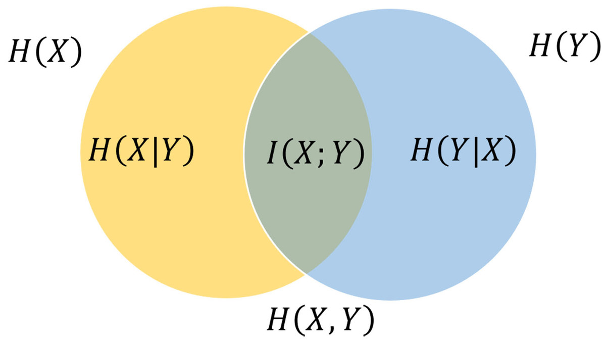
Figure 1: Venn diagram (Cover, 1999) shows additive and subtractive associations among diverse information metrics pertaining to correlated variables X and Y.
The joint entropy contains the area contained by either circle. The left circle symbolizes the individual entropy , where the crescent-shaped denotes the conditional entropy . The right circle signifies , with the crescent-shaped representing . The intersection between these circles denotes the mutual information .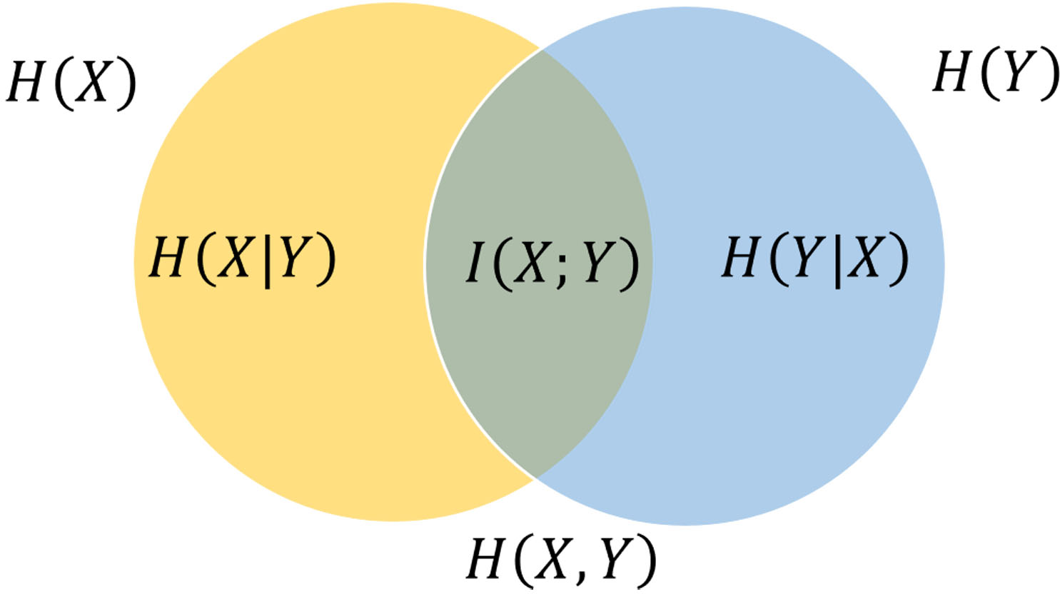
Substituting Eqs. (1) and (3) into (4) yield: (5) where is the joint PDFs of X and and are the PDFs of X and Y, respectively.
Conditional mutual information
Conditional mutual information is the formal definition of the mutual information between two random variables when conditioned on a third variable, as illustrated in Fig. 2. For jointly discrete random variables, this definition can be expressed as follows: (6)
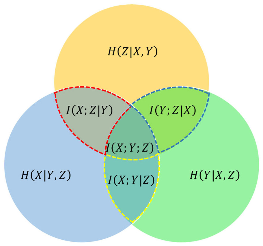
Figure 2: Venn diagram of information-theoretic measures for three variables X, Y, and Z, represented by the lower left, lower right, and upper circles, respectively.
The conditional mutual information , , and are represented by the red dotted line, blue dotted line, and yellow dotted line, respectively.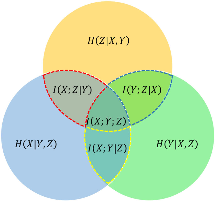
Substituting Eqs. (5) into (6) yield: (7)
In the context of discrete variables, Eq. (7) has been employed as a fundamental building block for establishing various equalities within the field of information theory.
Transfer entropy
Transfer entropy serves as a non-parametric statistical metric designed to quantify the extent of directed (time-asymmetric) information transfer between two stochastic processes (Schreiber, 2000; Seth, 2007). TE provides an information-theoretic methodology for evaluating causality by quantifying uncertainty reduction. According to Schreiber (2000), the TE from a stationary time series X to Y is defined as: (8) where, X and Y denotes the historical information of X and Y. It indicates that Eq. (8) is a special CMI (Wyner, 1978; Dobrushin, 1963) in Eq. (6) with the history of the influenced variable Y in the condition, which is used widely in practice.
Substituting Eqs. (7) into (8) yield: (9) where p means the PDFs, , τ represents the sampling period, and h denotes the prediction horizon. k signifies the embedding dimension for variable yi and d represents the embedding dimension for variable xj.TEX→Y from X to Y can be conceptualized as the improvement gained by using the historical data of both X and Y to forecast the future of Y, as opposed to solely relying on the historical data of Y alone. Essentially, it measures the information regarding an upcoming observation of variable Y obtained from the simultaneous observations of past values of both X and Y, while subtracting the information solely derived from Y’s past values concerning its future.
In a more detailed context, given two random processes and gauge the quantity of information using Shannon entropy (Shannon, 1948), the TEX→Y can be expressed as: (10) where H is the Shannon entropy of X.
Derived from Eqs. (9) or (10), an indirect causality topology based on multivariate time series can be obtained, as shown in Fig. 3.
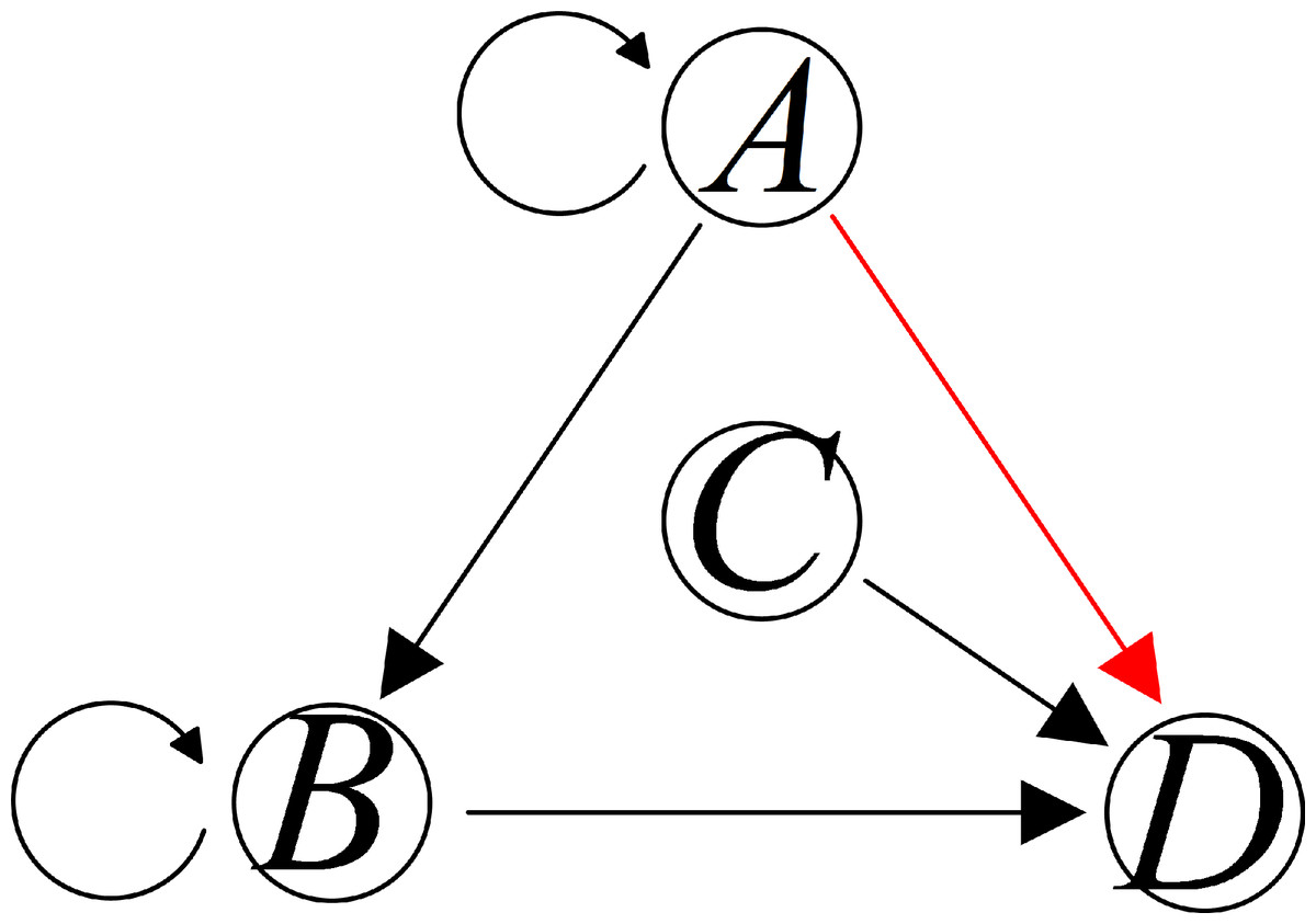
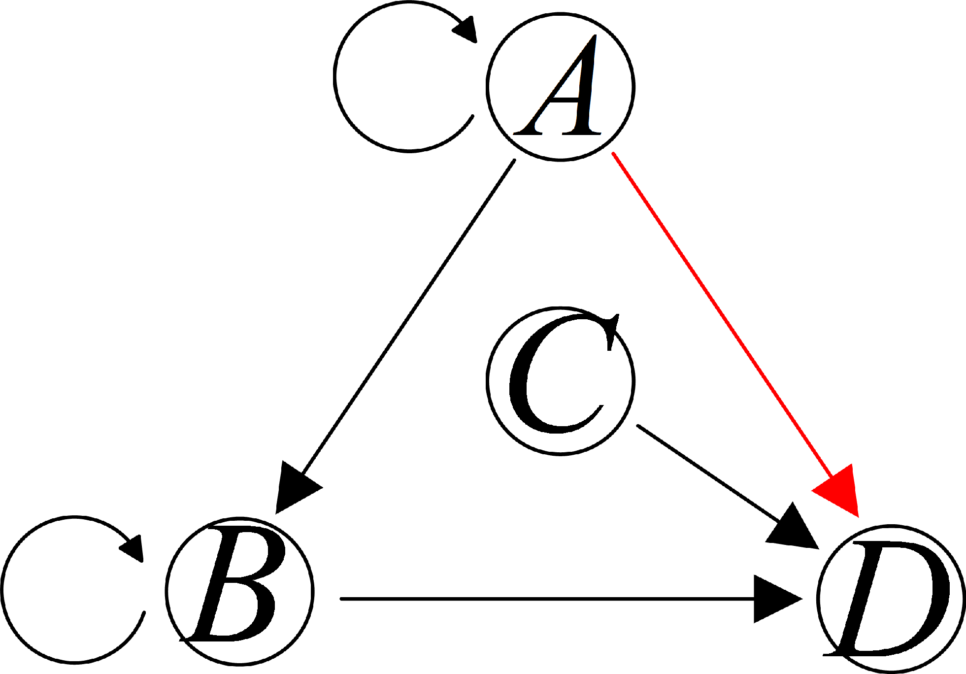
Figure 3: Two different patterns of causality topology between variables A, B, C, and D.
Consider four processes denoted as A, B, C, and D, as illustrated in Fig. 3. Suppose the TE method uncovers a causal influence from A to D. Within this context, two distinct causal patterns exist from A to D. However, it is essential to note that the TE, as described in Eqs. (9) or (10), is unable to distinguish whether this impact is direct or if it is transmitted through B. In other words, the TE lacks the capability to differentiate between a direct causality relationship and an indirect one. Additional methods must be incorporated to address the need for an equivalent underlying model to capture direct causality.
Conditional transfer entropy
In a complex system, it is not always guaranteed that TE exclusively represents the directed causal influence from X to Y. Information shared between X and Y may be conveyed through an intermediary third process, denoted as Z. In such scenarios, the presence of this shared information can lead to an augmentation in TE, potentially confounding the causal interpretation. One possible approach is conditional transfer entropy, which reduces the influence of shared information through alternative processes. CTE from a single source X to the target Y, while excluding information from Z, is then defined as follows: (11) where n represents the embedding dimension for variable zl.
In the case mentioned in Fig. 3, the direct causality relationship can be distinguished from the indirect one via the CTE method to capture the direct causal topology. When the causal impact from A to D is entirely conveyed through B, CTEA→D|B is uniformly zeros theoretically, which means that the addition of past measurements of A, contingent on B, will not enhance the prediction of D any further. Conversely, when there exists a direct influence from A to D, incorporating past measurements of A alongside those of B and D leads to enhanced predictions of D, resulting in a causal effect CTEA→D|B > 0.
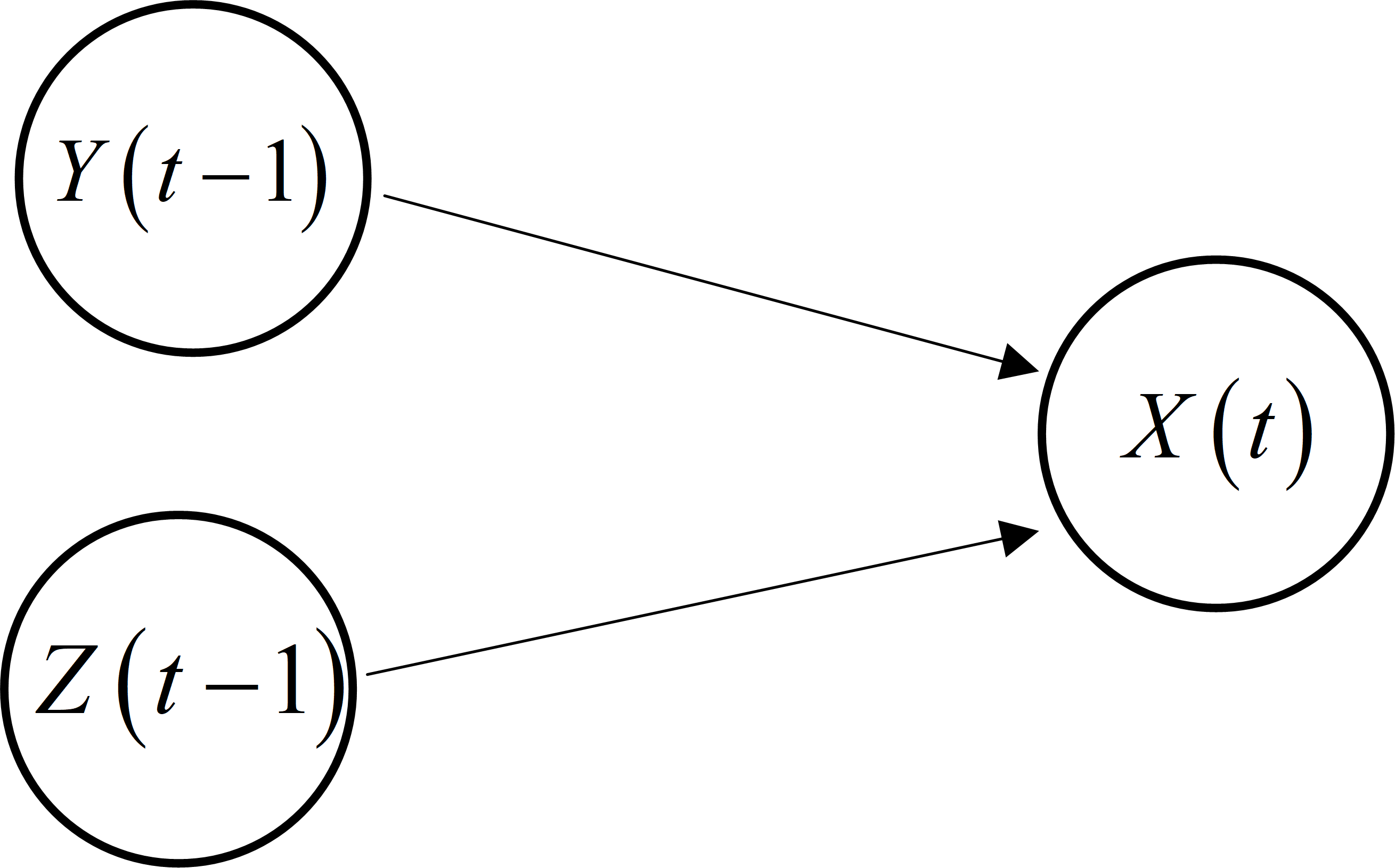
Utilizing MI in Eq. (5), CMI in Eq. (7), TE in Eq. (9), and CTE in Eq. (11), a set of foundational elements derived from the direct causality topology. Given four variables A, B, C, and D, suppose that the direct causal inference can be obtained, as shown in Fig. 4.
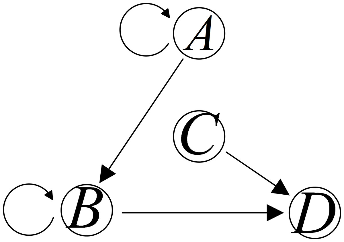
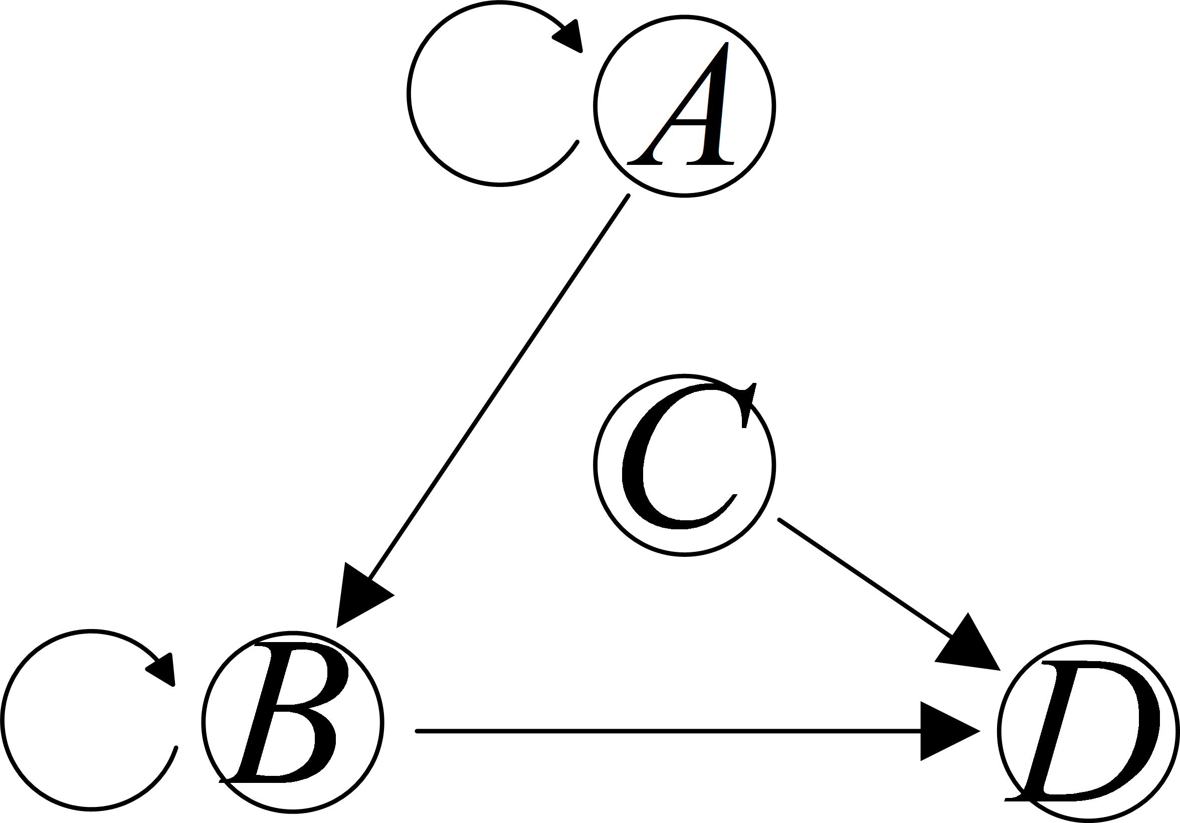
Figure 4: Direct causality topology between variables A, B, C, and D.
Derived from the direct causality topology depicted in Fig. 4, we can ascertain the sets of fundamental elements associated with each variable. The equivalent foundational model can be articulated as follows: (12) where each represents the equivalent underlying model of variable i, i = A, B, C, D. x signifies a collection of fundamental elements corresponding to variable i. For instance, consider the case where . Here, presents the measurements of C at sampling stamp t − 1 and t − 2, directly contributing to the causal relationship to D. It is worth noting that x can be determined through MI, TE, CMI, and CTE methods. In the subsequent section, the parameters and order of the functions fi will be determined using a polynomial fitting approach.
Significance test
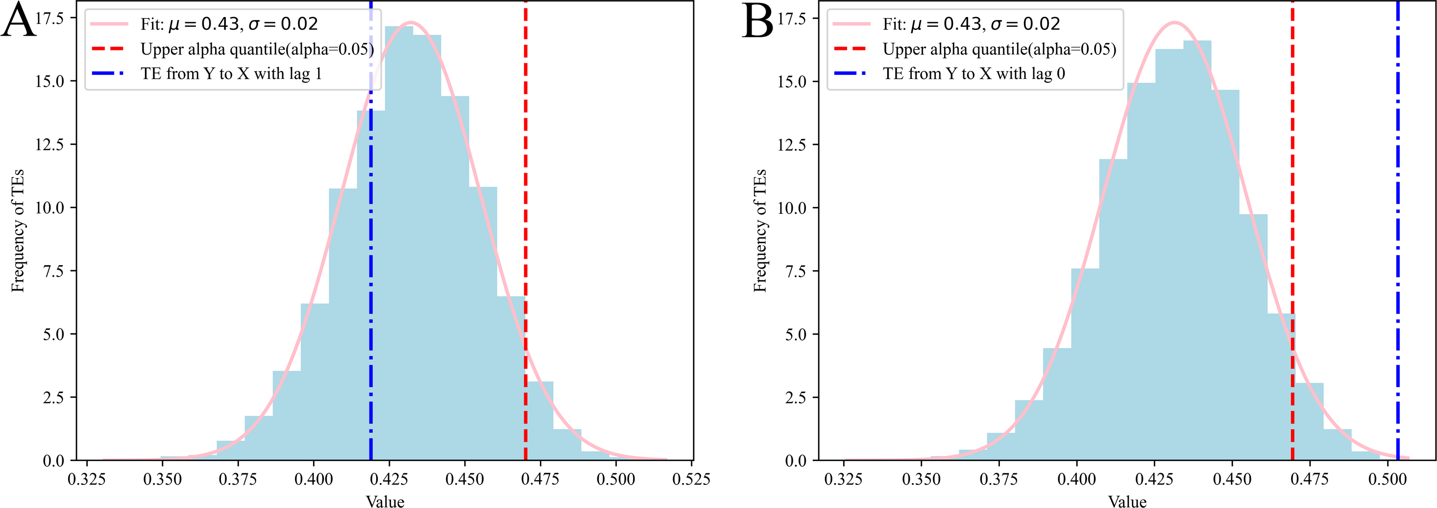
By conducting N-trial Monte Carlo simulations (Kantz & Schreiber, 2004), we compute the MIs, TEs, CMIs and CTEs for various surrogate time series, following Eqs. (5), (9), (7) and (11). These surrogate time series are randomly generated, and any potential causality between the time series is intentionally removed. In Fig. 5, the TEs for 10,000 pairs of uncorrelated random series are presented (partial results are presented here, with all results displayed in Supplemental Information). The results suggest that the MIs, TEs, CMIs and CTEs derived from the surrogate data demonstrate a Gaussian distribution, represented as . If we denote the MIs, TEs, CMIs and CTEs as random variables X, the PDF can generally be expressed as follows: (13) where the parameter µrepresents the expected value of the distribution, while the parameter σ denotes its standard deviation. The variance of the distribution is expressed as σ2. Let , the PDF of Z can be written as: (14)
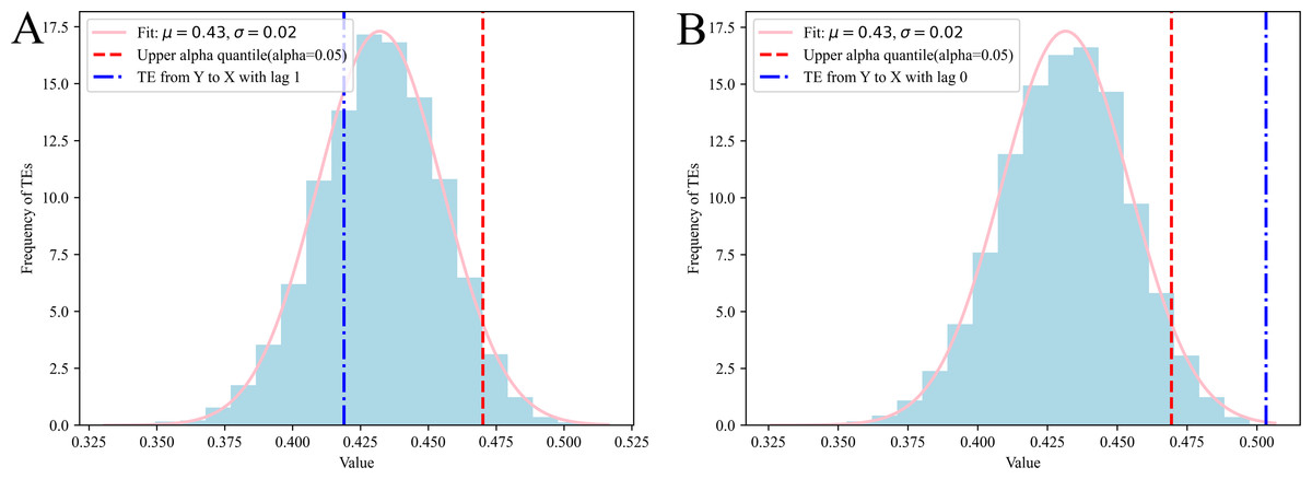
Figure 5: TEs from white Gaussian noise to a specific variable with lag, derived from N-trial Monte Carlo simulations, in case 1.
The cumulative distribution function (CDF) of the standard normal distribution, typically denoted by the capital Φ, is defined as the integral: (15)
There exists α > 0 such that: (16)
The quantile of the standard normal distribution is frequently symbolized as zα. A normal standard random variable will lie beyond the bounds of the confidence interval with probability α, which is a small positive number, often 0.05, denoting as z0.05. It means that 95% of the MIs, TEs, CMIs and CTEs derived from uncorrelated random series should be included in . We could also say that with 95% confidence, we reject the null hypothesis that the MIs, TEs, CMIs and CTEs are insignificant. Therefore, if or , it implies a noteworthy connection between variable X and Y. Moreover, if TEX→Y > z0.05 or , it implies a noteworthy causal connection from variable X to Y. Meanwhile, TEX→Y|Z > z0.05 or , it indicates a significant causality from variable X to Y, excluding information from Z. Additionally, if or , it indicates a significant connection between variable X and Y, excluding information from Z. It should be noted that the value of z0.05 depends on the specific distribution.
Polynomial fitting
The polynomial fitting method, employing a maximum exponent of k for each input feature, utilizes to create a polynomial features matrix A. This matrix comprises features, consequently leading to the establishment of a linear system: (17) where B is the coefficients and intercept. The Eq. (17) can be effectively solved using the “preprocessing.PolynomialFeatures” and “linear_model.LinearRegression” classes within the Python package “sklearn”.
Simulation Study
In this section, two cases are given to show the usefulness of the proposed method. The initial situation pertains to a basic discrete-time dynamical system representing a mathematical model. The second case is the Henon map, which illustrates dynamic systems exhibiting chaotic behavior.
Case 1: simulation case
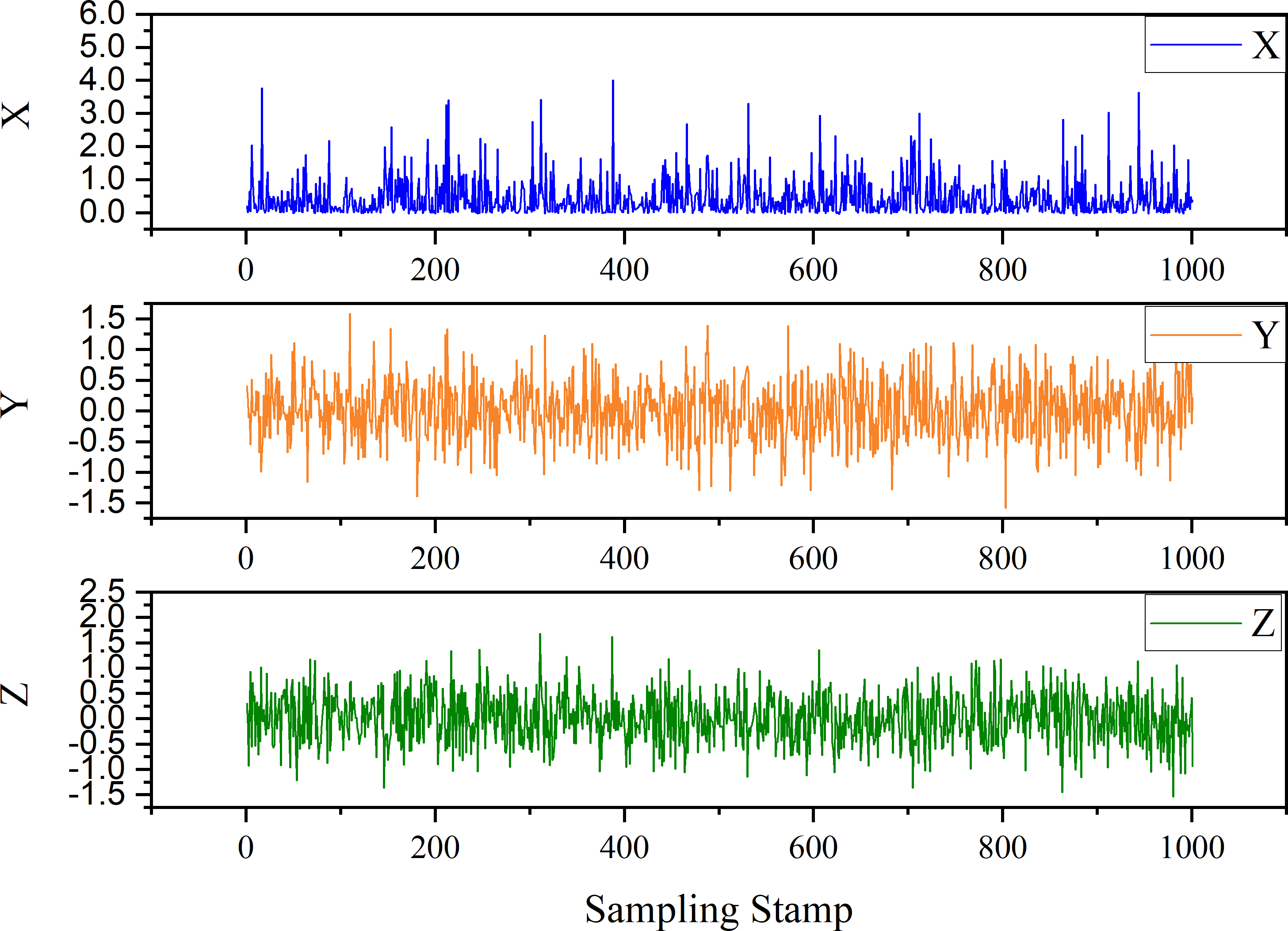
In the first instance, we have a discrete-time dynamical system. The expression is as follows: (18) where the two parameters are σ = 0.9, ρ = 0.7, and . The initial conditions are X(0) = 0.2, Y(0) = 0.4, and Z(0) = 0.3. The , where i = 1, 2, 3, represent the White Gaussian Noise. The trend generated by the time series derived from Eq. (18) is shown in Fig. 6.
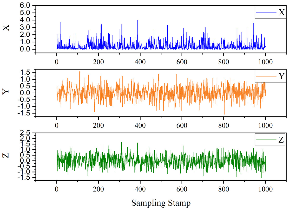
Figure 6: Trend of case 1.
Table 1 presents a comprehensive overview of TEs between each pair of variables with their respective time lags. In this table, p denotes the probability and the z0.05, upper α quantile (α = 0.05), serves as the upper boundary of the confidence interval.
| Cause | Effect | lag = 1 | lag = 2 | ||||
|---|---|---|---|---|---|---|---|
| TEcause→effect | z0.05 | p(α = 0.05) | TEcause→effect | z0.05 | p(α = 0.05) | ||
| X | Y | 0.5566 | 0.8873 | 1 | 0.5474 | 0.8891 | 1 |
| X | Z | 0.5712 | 0.9245 | 1 | 0.5695 | 0.9253 | 1 |
| Y | X | 0.5033 | 0.4694 | 0.0009 | 0.4189 | 0.4701 | 0.7172 |
| Y | Z | 0.8402 | 0.9254 | 0.6417 | 0.8345 | 0.9257 | 0.6987 |
| Z | X | 0.5247 | 0.4697 | 0 | 0.4385 | 0.4692 | 0.3841 |
| Z | Y | 0.8292 | 0.8879 | 0.4132 | 0.8128 | 0.8891 | 0.5876 |
The causality topology, derived from Tables 1 and 2 through TE and MI analysis, is visually depicted in Fig. 7. Notably, it becomes evident that there is only one unique pattern of causality between each pair of variables, each associated with their respective time lags. In other words, there is no presence of indirect causal influence. Consequently, the equivalent underlying model can be succinctly expressed as follows: (19)
| Cause | Effect | lag = 1 | lag = 2 | ||||
|---|---|---|---|---|---|---|---|
| z0.05 | p(α = 0.05) | z0.05 | p(α = 0.05) | ||||
| X | X | 0.0919 | 0.1341 | 0.9947 | 0.0975 | 0.1340 | 0.9756 |
| Y | Y | 0.1517 | 0.1644 | 0.2670 | 0.1576 | 0.1645 | 0.1385 |
| Z | Z | 0.1309 | 0.1633 | 0.8454 | 0.1447 | 0.1638 | 0.4595 |

Figure 7: Causality topology between each pair of variables with their respective time lags.
In the subsequent step, we employ polynomial approximation to estimate the genuine underlying model. The parameters and order of the equivalent fX are determined through the polynomial fitting approach as outlined in Eq. (18). In this process, we opt for a higher order k for fX: (20) where , B = [b0,0], [b1,0, b0,1, b2,0, b1,1, b0,2⋯, b1,k−1, b0,k]T. When selecting k = 4, these parameters can be obtained by fitting, b0,4 = 3.2∗10−3, b1,3 = 3.2∗10−3, b2,2 = − 3.2∗10−3, b3,1 = − 4.8∗10−3, b4,0 = 2.1∗10−3, b0,3 = − 3.4∗10−3, b1,2 = − 6.8∗10−3, b2,1 = − 2.9∗10−3, b3,0 = 7.7∗10−4, b0,2 = 0.93, b1,1 = 1.9, b2,0 = 0.9, b0,1 = 2.4∗10−3, b1,0 = 1.5∗10−3, b0,0 = 1.9∗10−4. Disregarding coefficients that are insignificantly close to zero, the expression in Eq. (20) can be redefined as follows: (21)
It is evident that the underlying model in Eq. (18) can be concisely represented by Eq. (21). The training dataset consists of 700 samples in our experimental configuration, while the testing dataset comprises 300 samples. Figure 8 elegantly showcases the fitting curves of the time series achieved through the proposed method. Remarkably, when supervised, the original series and the polynomial fit data (derived from the equivalent underlying model) exhibit an exceptionally close alignment. In contrast, without supervision, the performance is significantly reduced. This reduction in performance is likely attributed to and relying solely on white Gaussian noise, which exhibits a considerable degree of randomness.
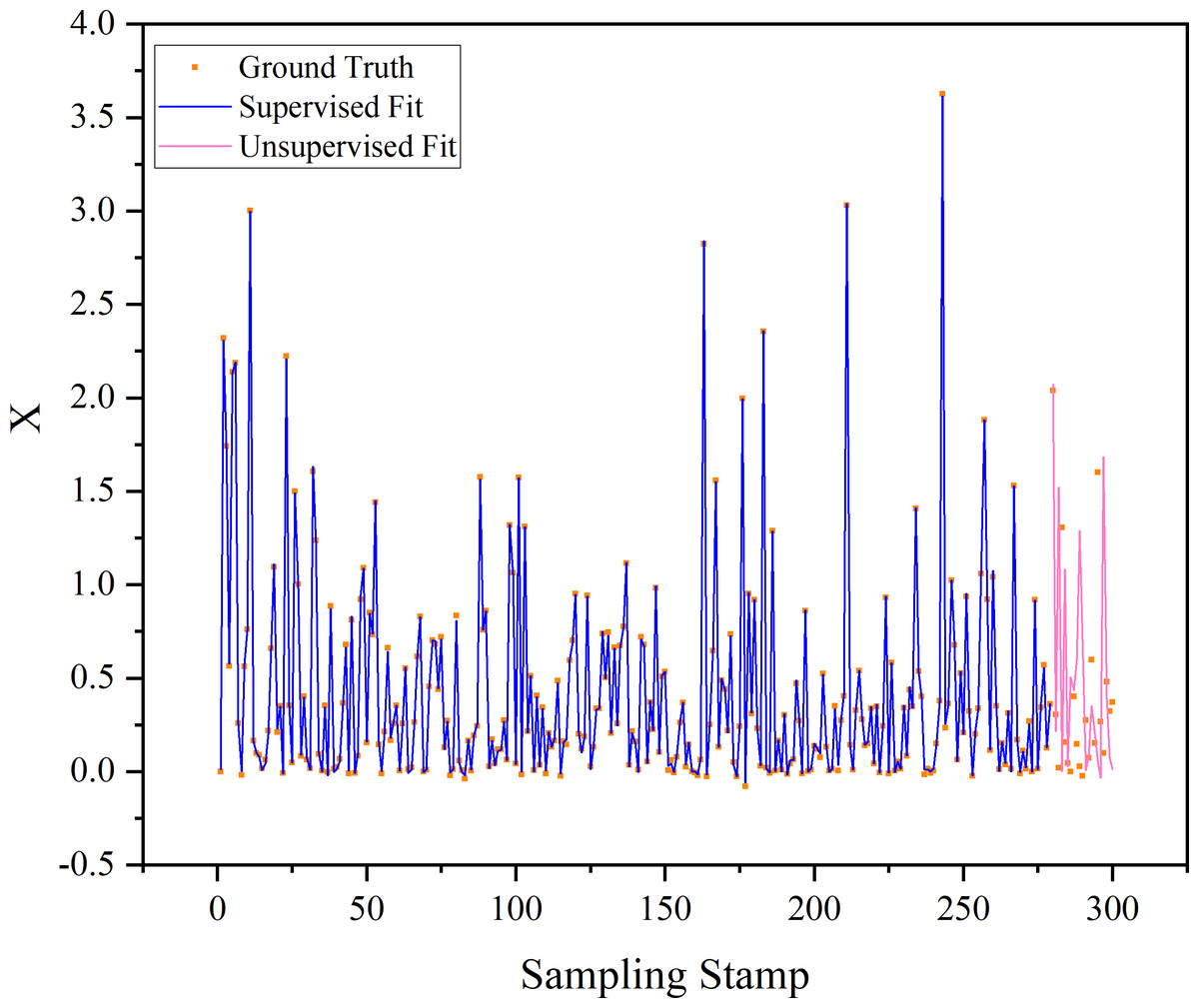
Figure 8: Fitting curves of time series based on the proposed method.
The “supervised fit” signifies that each input is derived from the Ground Truth to compute the current output. In contrast, “unsupervised fit” denotes that an initial input is provided, and all outputs are calculated through iterative processes without relying on Ground Truth.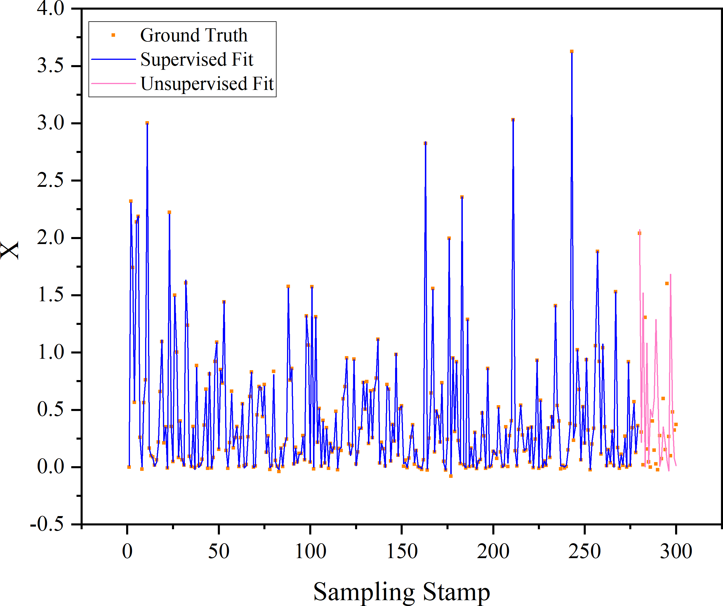
Case 2: Henon map chaotic time series
The Henon map constitutes a discrete-time dynamical system characterized by chaotic behavior. Here is the expression of the Henon map system: (22) where the parameters α and β are set to α = 1.4 and β = 0.3, respectively, while the initial states are X(0) = 0 and Y(0) = 0. The trend generated by the time series derived from Eq. (22) is shown as Fig. 9.
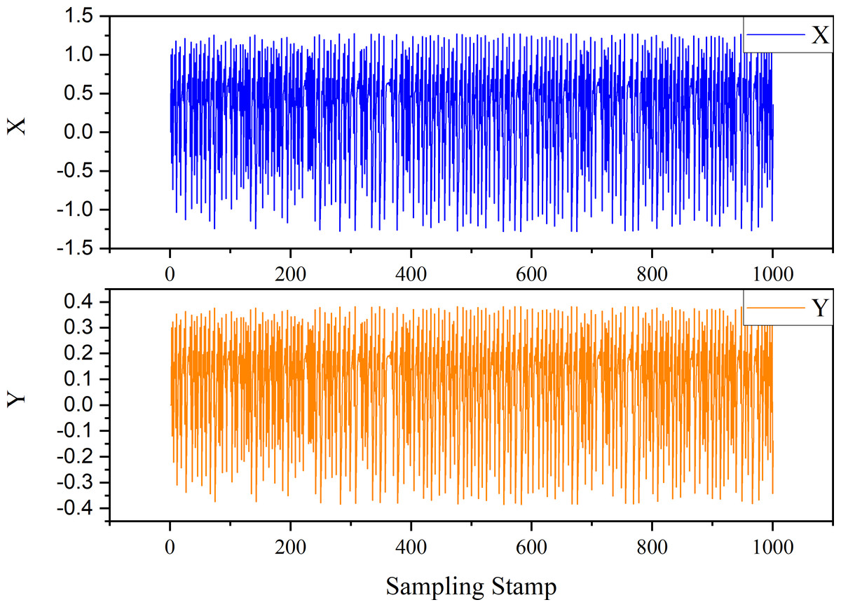
Figure 9: Trend of case 2.
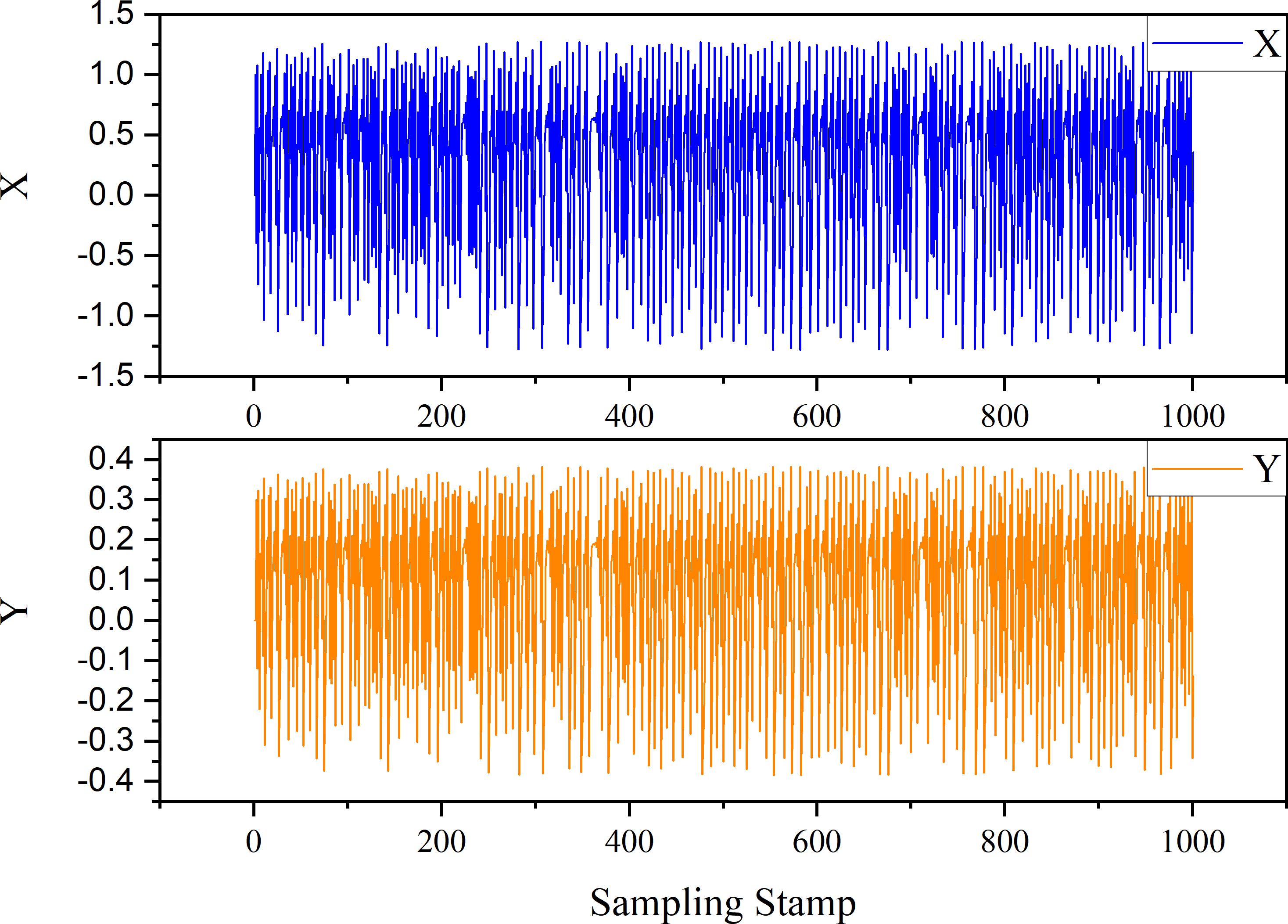
Table 3 presents a comprehensive overview of TEs between each pair of variables with their respective time lags. Notably, the TE method has detected the causal influences from to , to , to .
| Cause | Effect | lag = 1 | lag = 2 | ||||
|---|---|---|---|---|---|---|---|
| TEcause→effect | z0.05 | p(α = 0.05) | TEcause→effect | z0.05 | p(α = 0.05) | ||
| X | Y | 1.3323 | 0.4866 | 0 | 0.0093 | 0.4842 | 1 |
| Y | X | 0.7191 | 0.4823 | 0 | 0.7068 | 0.4804 | 0 |
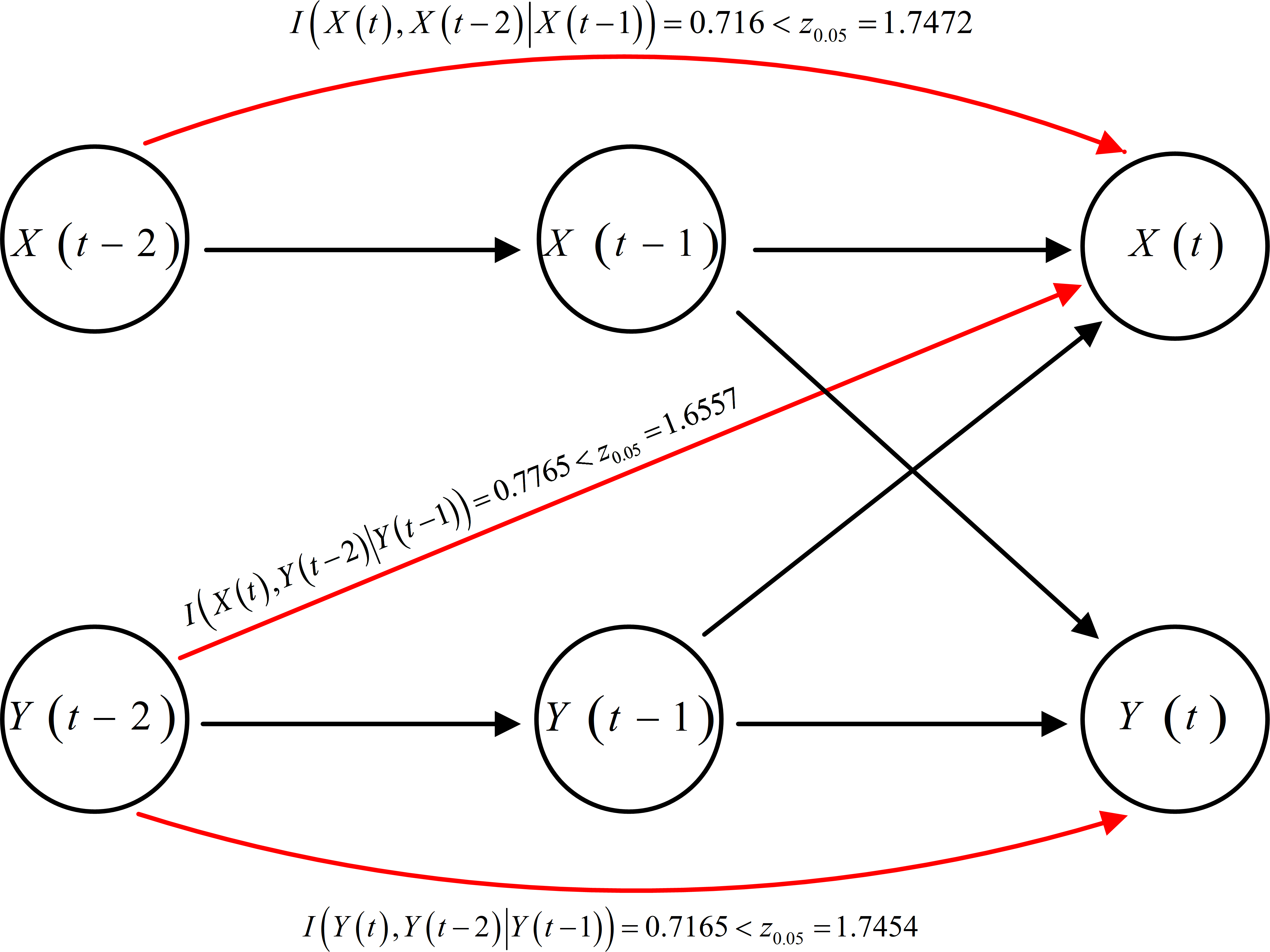
The causality topology, derived from Tables 3 and 4 through both TE and MI analyses, is visually represented in Fig. 10. Notably, there exist two types causal influences, direct and indirectly, among the following three pairs of variables: to , to , and to . To further investigate these causal relationships and distinguish whether the influence is direct or mediated by three, we employ CMI or CTE to capture direct causality.
| Cause | Effect | lag = 1 | lag = 2 | ||||
|---|---|---|---|---|---|---|---|
| z0.05 | p(α = 0.05) | z0.05 | p(α = 0.05) | ||||
| X | X | 1.5725 | 0.1938 | 0 | 1.2878 | 0.1942 | 0 |
| Y | Y | 1.569 | 0.1939 | 0 | 1.2801 | 0.1942 | 0 |
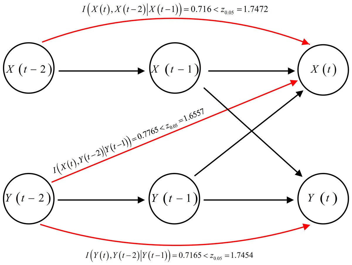
Figure 10: Causality topology between each pair of variables with their respective time lags.
Each of these three undetermined causal relationships involves its historical measurements. Consequently, the CMI is more suitable for distinguishing whether a third variable’s influence is direct or mediated. The outcomes of the analysis using CMI are outlined in Table 5. The results indicate that these causal relationships are indeed direct rather than indirect. This implies that the red arrows should be removed, and the rest of the diagram reflects the direct causal topology (shown in Fig. 10).
| Cause | Effect | Condition | z0.05 | p(α = 0.05) | |
|---|---|---|---|---|---|
| 0.7160 | 1.7472 | 1.0 | |||
| 0.7765 | 1.6557 | 1.0 | |||
| 0.7165 | 1.7454 | 1.0 |
Consequently, the equivalent underlying model can be succinctly expressed as follows: (23)
In the subsequent step, we employ polynomial approximation to estimate the genuine underlying model. When choosing k = 4, these parameters of fX can be obtained by fitting. b0,0 = 1, b0,1 = 1, b2,0 = − 1.4, and the rest of the coefficients are insignificantly close to zero, one expression in Eq. (23) can be redefined as follows: (24)
Similarly, another the expression in Eq. (23) can be redefined as follows: (25)
The underlying model of the Henon map can be concisely represented by Eqs. (24) and (25). Within our experimental configuration, the training dataset consists of 700 samples, while the testing dataset comprises 300 samples. Figure 11 elegantly portrays the fitting curves of the time series achieved through the proposed method. Both supervised and unsupervised cases exhibit an exceptionally close alignment between the original series and the polynomial fit data derived from the equivalent underlying model. This outcome is likely due to and not relying on White Gaussian Noise, thereby reducing the influence of randomness.
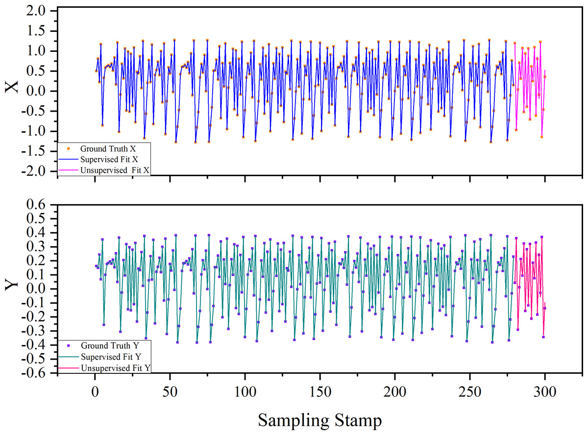
Figure 11: Causality topology between each pair of variables with their respective time lags.
The “supervised fit” signifies that each input is derived from the Ground Truth to compute the current output. In contrast, “unsupervised fit” denotes that an initial input is provided, and all outputs are calculated through iterative processes without relying on Ground Truth.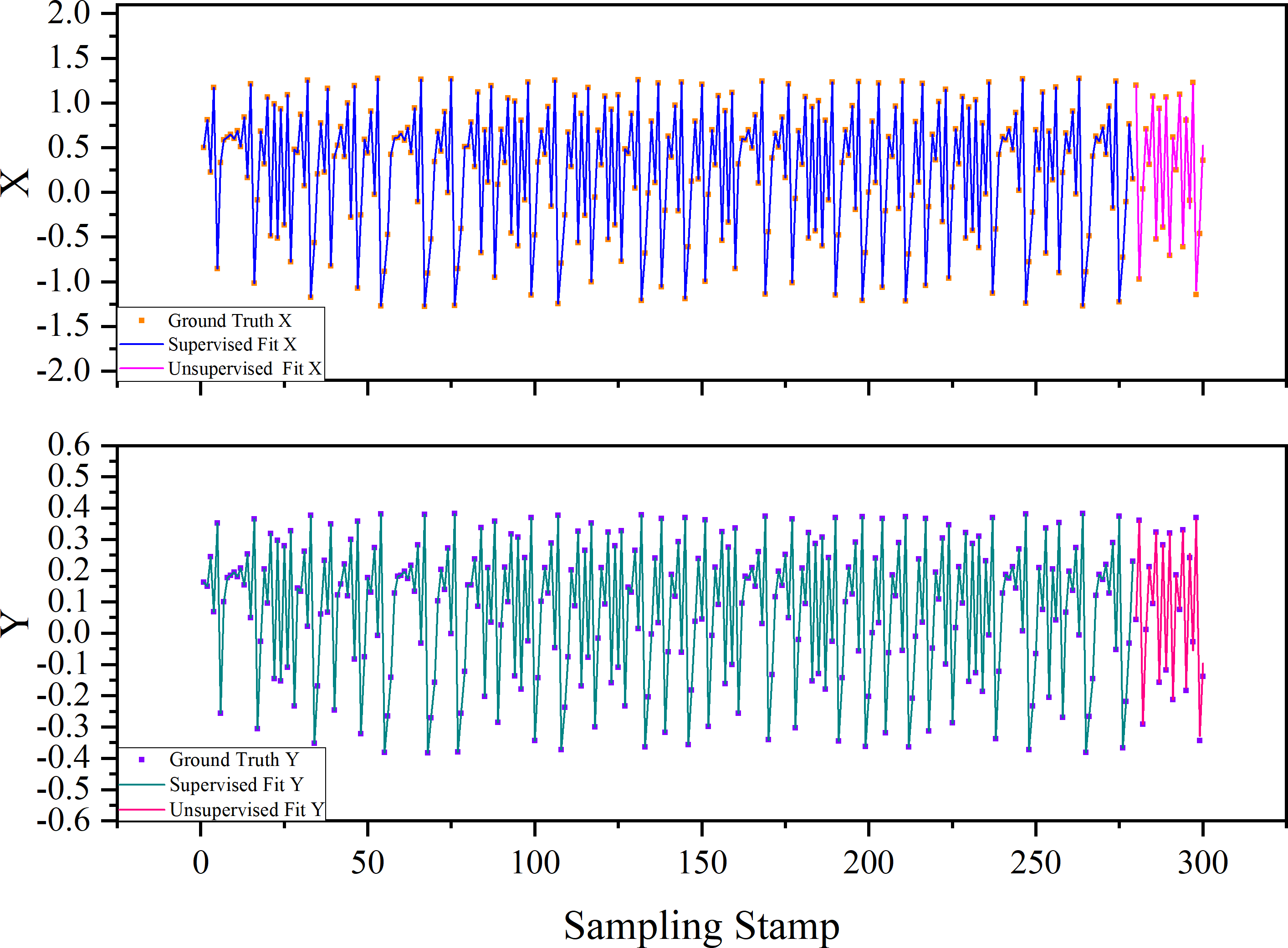
Conclusions
This article introduces an innovative and effective method for reconstructing an equivalent underlying model, built upon the direct causality topology derived from multivariate time series data. MI and TE are utilized to map out the causality structure, whereas CMI or CTE is employed to distinguish between direct causal influences and indirect ones. By employing the polynomial fitting method, we are able to derive the expression of the equivalent underlying model solely based on the direct topology without the need for prior knowledge. This method provides a systematic and data-driven approach for uncovering the inherent causal structures within multivariate time series data. It allows for accurately identifying and reconstructing an equivalent underlying model, enhancing our understanding and interpretation of complex systems represented in the data. This study focuses on reconstructing an equivalent underlying model that primarily identifies dynamic systems. This approach can be seamlessly adapted for other applications, including correlation and causality analysis. Moving forward, our objective is to refine these reconstructed models further. This work includes integrating AI and machine learning techniques to enhance the accuracy and efficiency of the models and expand their applicability across diverse domains.
Supplemental Information
Equivalent underlying model data
Case 1 is a discrete-time dynamical system. Case 2 is a Henon map chaotic time series. For each case, the training dataset consists of 700 samples, while the testing dataset comprises 300 samples.