
Steganography in color images with random order of pixel selection and encrypted text message embedding
- Published
- Accepted
- Received
- Academic Editor
- Robertas Damaševičius
- Subject Areas
- Algorithms and Analysis of Algorithms, Cryptography, Multimedia, Security and Privacy
- Keywords
- Steganography, Text encryption, Color images steganography, Least-significant bit steganography, Steganographic analysis
- Copyright
- © 2021 Kordov and Zhelezov
- Licence
- This is an open access article distributed under the terms of the Creative Commons Attribution License, which permits unrestricted use, distribution, reproduction and adaptation in any medium and for any purpose provided that it is properly attributed. For attribution, the original author(s), title, publication source (PeerJ Computer Science) and either DOI or URL of the article must be cited.
- Cite this article
- 2021. Steganography in color images with random order of pixel selection and encrypted text message embedding. PeerJ Computer Science 7:e380 https://doi.org/10.7717/peerj-cs.380
Abstract
Information security is major concern in modern digital ages, and the outdated algorithms need to be replaced with new ones or to be improved. In this article a new approach for hiding secret text message in color images is presented, combining steganography and cryptography. The location and the order of the image pixels chosen for information embedding are randomly selected using chaotic pseudo-random generator. Encrypting the secret message before embedding is another level of security designed to misguide the attackers in case of analyzing for traces of steganography. Evaluating the proposed stegoalgorithm. The standard statistical and empirical tests are used for randomness tests, key-space analysis, key-sensitivity analysis, visual analysis, histogram analysis, peak signal-to-noise ratio analysis, chi-square analysis, etc. The obtained results are presented and explained in the present article.
Introduction
Steganology is an ancient science that is becoming more and more widely used with the development of digital information.
It consists of two main areas: steganography and steganalysis. Steganography is an interdisciplinary applied science field (Cox et al., 2007; Stanev & Szczypiorski, 2016), a set of technical skills and art for ways to hide the fact of transmission (presence) of information. It is one of the most effective approaches to protecting important information by hiding it (data hiding). High-tech steganography summarizes the areas for hiding messages using communication and computer technology, nanotechnology and modern advances in sciences such as biology, chemistry and others (Wu et al., 2020; Koptyra & Ogiela, 2020; Abd-El-Atty et al., 2020).
Steganalysis has exactly the opposite task. It combines methods and technologies for detecting secret steganographic communications. Along with the beginning of the development of modern ways of hiding information, at the end of the 20th century research in the field of steganalysis (Johnson & Jajodia, 1998; Provos & Honeyman, 2001; Fridrich & Goljan, 2002) has begun. Steganalysis is divided into two main categories: blind and targeted (Zhelezov, 2016). Targeted steganalysis methods have been developed to detect data embedded with specific stegoalgorithms and they are very accurate against certain stegomethods. The blind analysis methods are based on algorithms that require prior “training” with a series of empty and filled containers. The most characteristic of both types of analysis is that their methods are based on statistical dependencies in the analyzed subjects (Nissar & Mir, 2002). Such a method is POV (Pairs of Values) as part of the chi-square analysis (Westfeld & Pfitzmann, 1999; Fridrich, Goljan & Du, 2001).
Related work
One of the latest research which shows successful Optical Character Recognition (OCR) steganography technique with good results in steganalysis, is presented in (Chatterjee, Ghosal & Sarkar, 2020). Other example of resent steganographic research is described in (Pak et al., 2020), where the authors are using chaotic map for constructing a steganographic algorithm. Popular methods for image steganography are analyzed in Table 1.
| Reference | Marvel, Boncelet & Retter (1999) |
| Method | The method uses a fast compressed-domain embedding technique to facilitate on-the-fly |
| compressed-domain public-key steganography | |
| Notes | Low probability of detection and leaving an observer unaware that the hidden data exist. |
| The method works with grayscale images | |
| Reference | Satish et al. (2004) |
| Method | The method is based on a scheme of chaos based spread spectrum image steganography (CSSIS) |
| involving the use of chaotic encryption and chaotic modulation in spread spectrum image | |
| steganography (SSIS) | |
| Notes | A novel scheme of the use of chaos based encryption. Robustness is achieved by interleaving |
| the message using a chaotic sequence | |
| Reference | Baby et al. (2015) |
| Method | The method is based on hiding multiple color images into a single color image using the |
| Discrete Wavelet Transform | |
| Notes | DWT increases the payload of the steganographic process by data compression. The proposed |
| approach provides a good PSNR and SSIM value which establish the robustness of this work | |
| Reference | Amirulhaqi, Purboyo & Nugrahaeni (2017) |
| Method | The method is based on Spread Spectrum Steganography and the Vigenere Cipher embedding |
| in gif images | |
| Notes | The method consists of three processes, namely the spreading, modulation, and insertion of a GIF image to the message |
| Reference | Yadav & Dutta (2017) |
| Method | The method is based on spread spectrum image steganography with RSA message encryption. |
| Notes | High level of security. Spreading the message all over the pixels of the cover media using pseudo |
| random generator that generates random locations of pixels in an image and embedding | |
| message with Least Significant Bit algorithm to make it highly indiscernible | |
| Reference | Gaurav & Ghanekar (2018) |
| Method | The method presents a steganography algorithm based on local reference edge detection |
| technique and exclusive disjunction in the sharp edge region compared to the uniform region | |
| of the image | |
| Notes | This paper presents an improved steganography technique on the basis of HVS system with |
| an improved XOR technique | |
| Reference | Chatterjee, Ghosal & Sarkar (2020) |
| Method | The method is based on Optical Character Recognition (OCR) based Steganographic technique. |
| Notes | Advantages—indicating correct classification by the model and high PSNR values. The method |
| works with grayscale images. Slow embedding process for large images | |
| Reference | Pak et al. (2020) |
| Method | The method is based on an improved 1D chaotic system model |
| Notes | The conventional one-dimensional (1D) chaotic map has a simple structure, which is easy to |
| implement and has a low computational cost. The algorithm shows a good performance against | |
| statistical analysis attacks. Conventional one-dimensional (1D) chaotic map has a drawback | |
| that the range of chaotic behaviors is narrow and the distribution of key sequence is uniform |
The main task of the steganographic algorithm is to reduce the efficiency of such methods and thus to increase its reliability. For this purpose, it is necessary to choose a method of embedding that does not violate the statistical dependencies.
For this reason, a Spread Spectrum Steganography approach (Marvel, Boncelet & Retter, 1999; Satish et al., 2004) based on a pseudo-random sequence generator has been chosen in this article. Additional text encryption is applied for transforming the secret message into unreadable character sequence for increasing the level of security of the proposed steganographic algorithm. In this approach, the resulting pseudo-random sequences are used to determine the message embedding positions. This leads to preserving the statistical dependencies in the container. Another advantage of this approach is related to some types of targeted steganalysis. They extract the values of the smallest bits of the file sequentially and analyze them for repetitive sequences. With the embedding method proposed in the article this type of steganalysis is completely ineffective.
Motivation and justification
The text messages and the digital images are the most used information carriers concerning the data flow in the Internet and mobile communications. There are thousand of chat applications designed for short text messages correspondence using different ways to secure the communications between the users. Variety of cryptographic algorithms are implemented in order to protect the transferred information. Unfortunately, some of the encryption methods have become outdated and the new ones are being invented to improve secure communication. Information security will always be a major concern that motivates the development of new secret methods for data distribution and real-time communication. Such method is proposed in this work by combining two general scientific areas: steganography and cryptography.
An outline of the proposed work
Our main focus is to present a different approach for classic LSB Steganography in images using random order of pixel selection and embedding encrypted text message. In order to achieve our goal the proposed technique requires the following steps:
-
constructing novel pseudo-random generator
-
secure text encryption, using the constructed pseudo-random generator
-
choosing random pixels (in chaotic order) from an image, using the constructed pseudo-random generator for embedding information
-
using traditional LSB pixel’s color modification for hiding, leaving no traces of steganography.
Pseudo-random Generator Based on Duffing Map and Circle Map
For random pixel selection we are using pseudo-random generator (PRG) described in this section. Pseudo-random generators (also called Pseudo-random number generators (PRNG)) are software realized and unlike True-random generators (TRG) are easy for implementation with significantly lower cost and time consumption. This is why they are often used in cryptographic and steganographic systems. Examples of PRGs can be found in (Kordov, 2014, 2015b). The requirement resistance of PRGs is to different types of attacks are discussed in this section.
Duffing map description
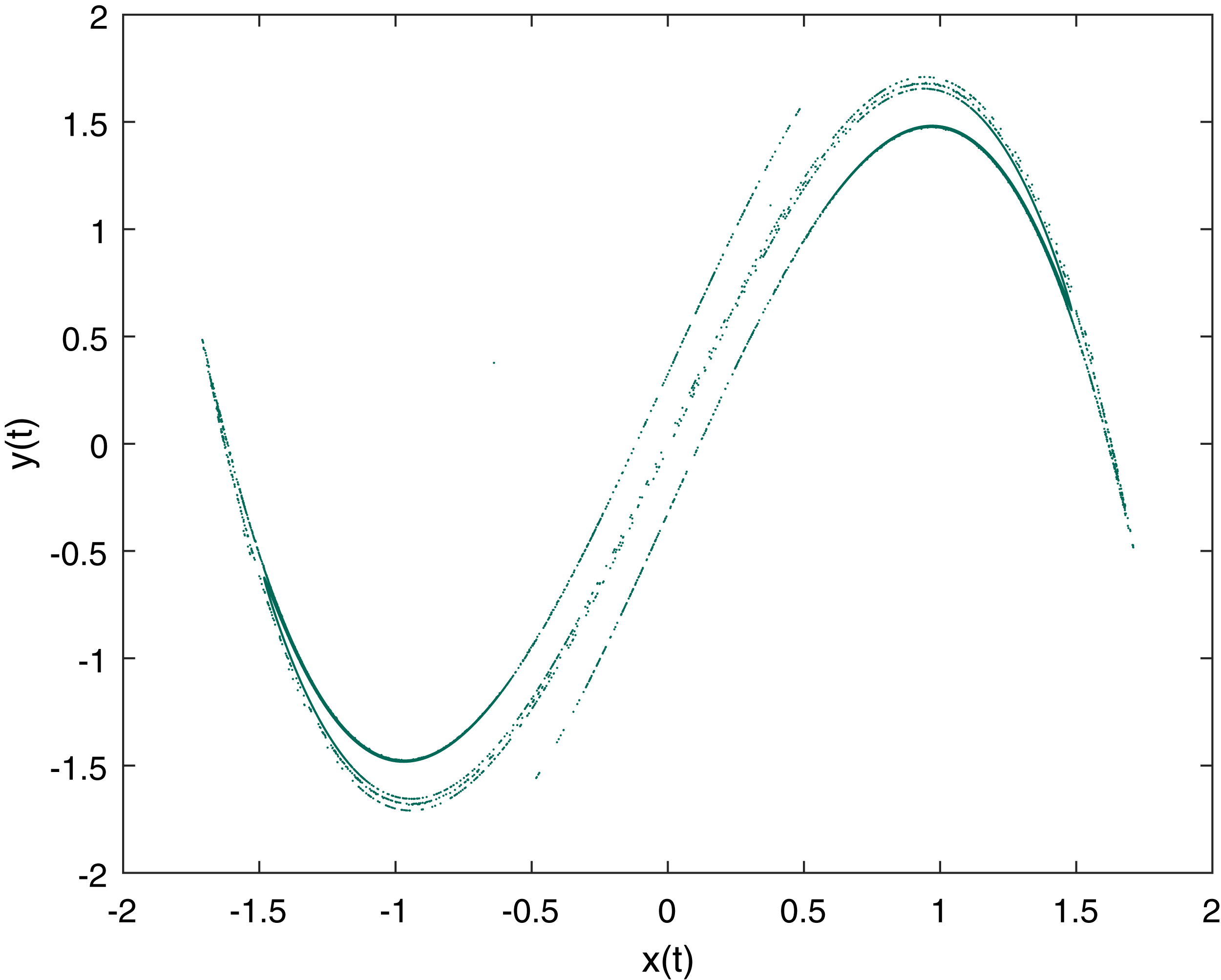
The Duffing map is well known two dimensional non-linear discrete-time dynamical system with chaotic behavior (Holmes & Moon, 1983) which is a discrete version of Duffing oscillator (Van Dooren, 1988). Duffing map is given by: (1) where xt and yt are double variables, calculated on every iteration, and a and b are fixed parameters of the Duffing map. For chaotic behavior the parameters are set to a = 2.75 and b = 0.2 (Hasan et al., 2017; Riaz et al., 2018). The initial test values we used for variables are x0 = −0.63825 and y0 = 0.37713 and Fig. 1 is a graphical representation of the Duffing map with the described values.
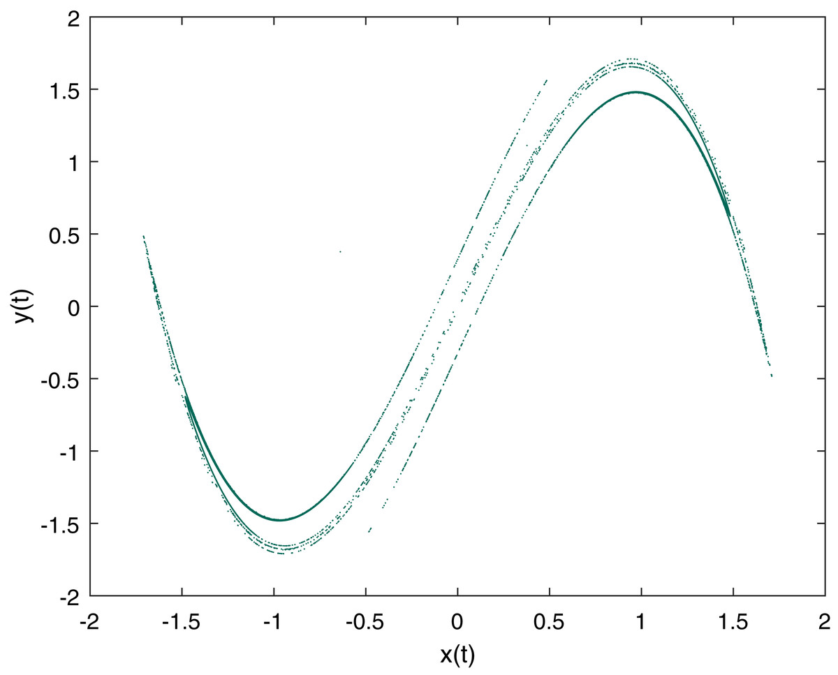
Figure 1: Duffing Map Plot with a = 2.75, b = 0.2, x0 = −0.63825 and y0 = 0.37713.
Circle map description
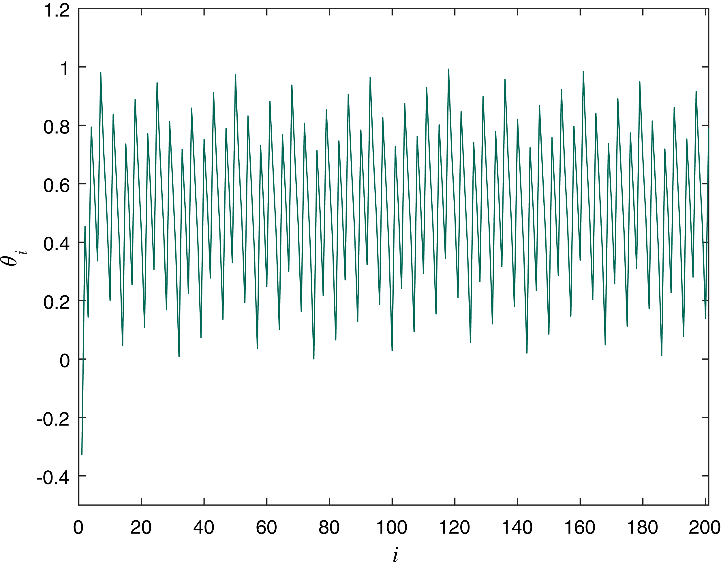
The Circle map is explored for chaotic behavior in Shenker (1982) and DeGuzman & Kelso (1991). It has random-like properties and is suitable for constructing PRGs (Kordov, 2015a). The Standard circle map equation is: (2) where θ is a double variable and Ω and K are the controlling parameters with values Ω = 0.7128281828459045, K = 0.5. The initial value for the variable we used for experiments in this article is θ0 = −0.329054. Figure 2 is a graphical representation of the Circle map with the described values.
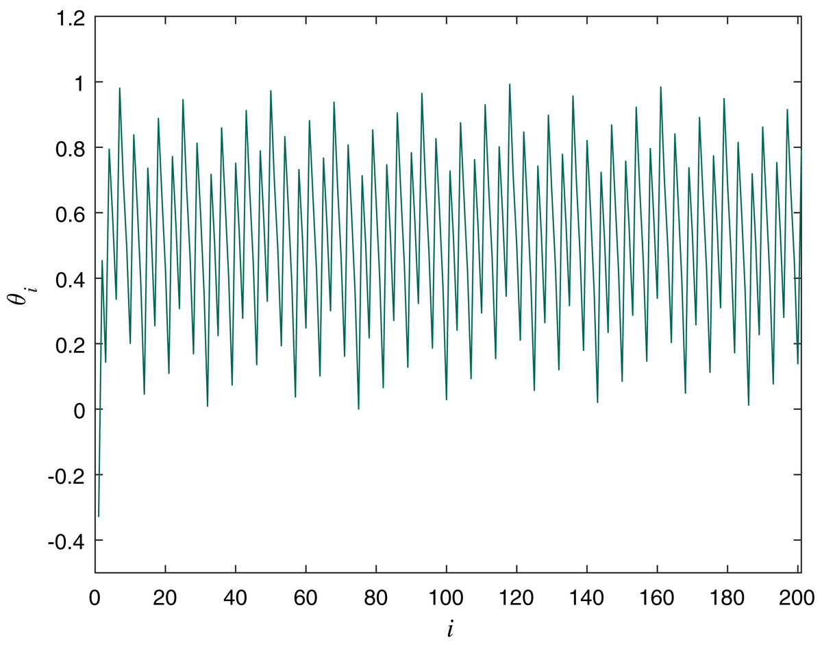
Figure 2: Circle Map Plot with Ω = 0.7128281828459045, K = 0.5 and θ0 = −0.329054.
Random bit extraction process
The proposed bit extraction process is using Eqs. (1) and (2) and contains the following steps:
-
The initial values of the constant parameters from Eqs. (1) and (2) are determined and the initial values of the double variables are set (described in the previous sections).
-
For additional security, first N iterations from Eq. (1) and first M iterations from Eq. (2) are skipped. (we randomly chose N = M = 541).
-
On every iteration of Eq. (1), xt and yt are used for calculation of additional double variable pt:
-
The produced random bit is obtained by performing XOR operation between the variables pt and qt.
-
The previous two steps are repeated until the necessary random binary sequence is reached.
Key-sensitivity analysis
This test is performed to determine the behavior of the proposed PRG if there are changes in the secret key that is used to produce binary sequences. To test the key sensitivity very similar secret keys are used (described in Table 2) by changing a single digit in one of the initial double variables.
| Secret | Variable values | ||
|---|---|---|---|
| Key | x0 | y0 | θ0 |
| K1 | −0.63825 | 0.37713 | −0.329054 |
| K2 | −0.63824 | 0.37713 | −0.329054 |
| K3 | −0.63826 | 0.37713 | −0.329054 |
| K4 | −0.63825 | 0.37712 | −0.329054 |
| K5 | −0.63825 | 0.37714 | −0.329054 |
| K6 | −0.63825 | 0.37713 | −0.329053 |
| K7 | −0.63825 | 0.37713 | −0.329055 |
The results of the experiment are graphically presented in Fig. 3 and clearly show that the final binary sequence is different every time even if the secret keys are very similar. This means the proposed PRG is very sensitive to any changes in the initial conditions.
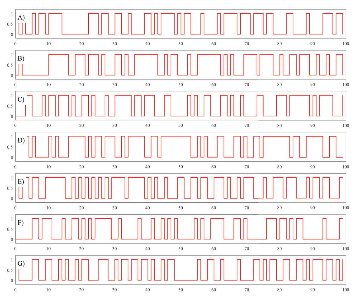
Figure 3: Circle Map Plot with Ω = 0.7128281828459045, K = 0.5 and θ0 = −0.329054.
(A) Plot of binary sequence using secret key K1. (B) Plot of binary sequence using secret key K2. (C) Plot of binary sequence using secret key K2. (D) Plot of binary sequence using secret key K3. (E) Plot of binary sequence using secret key K4. (F) Plot of binary sequence using secret key K5. (G) Plot of binary sequence using secret key K6.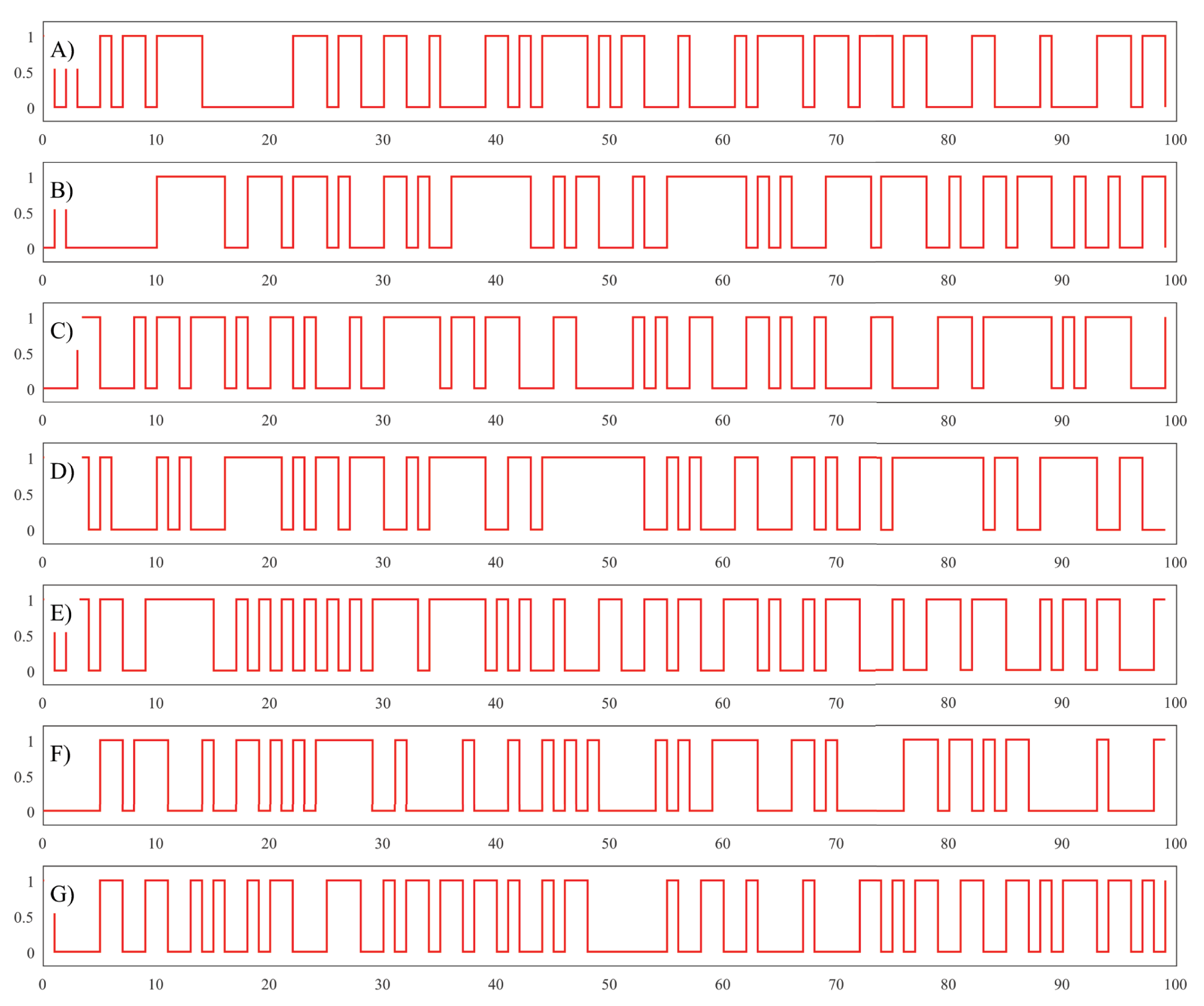
Key-space analysis
The key-space includes the variety of possible values of the used variables in random bit generation. Equation (1) has two initial variables that can have different values (x0 and y0) and Eq. (2) has one variable −θ0. The parameters from the equations are constant so they cannot be part of the secret key. In addition to the secret key, the integer values of N and M also can have different values. Considering the floating point standard of IEEE for double variables (IEEE Computer Society, 2008) every double variable has precision about 10−15. Combining the three variables we have (1015)3 ≈ 2149 plus (232)2 for the two integer variables and final about 2213 for key-space. The required key-space for resisting brute-force attacks is 2100 (Alvarez & Li, 2006) which means that the proposed PRG is secure enough. Kay-space comparison is presented in Table 3.
| Reference | Key-space |
|---|---|
| Kordov (2015a) | 2179 |
| Kordov (2014) | 2199 |
| Kordov (2015b) | 2199 |
| Proposed | 2213 |
Randomness evaluation
The most important property of a PRG is to produce random binary numbers. To evaluate the randomness 1 billion bits are generated and the sequence is tested with the most popular statistical test software packages.
NIST—random test
The first software for randomness evaluation is NIST—Statistical Test Suite (Bassham et al., 2010) and includes 17 base tests. The testing process is performed by dividing the tested sequence into 1,000 subsequences with length of 1,000,000 bits. All the NIST need to have P-values in the range [0,1) to be considered for successfully passed. The results for all tests are summarized in Table 4.
| NIST test | P-value | Pass rate |
|---|---|---|
| Frequency | 0.844641 | 991/1,000 |
| Block-frequency | 0.140453 | 993/1,000 |
| Cumulative sums (Forward) | 0.002820 | 993/1,000 |
| Cumulative sums (Reverse) | 0.723804 | 995/1,000 |
| Runs | 0.664168 | 991/1,000 |
| Longest run of Ones | 0.803720 | 996/1,000 |
| Rank | 0.473064 | 994/1,000 |
| FFT | 0.552383 | 991/1,000 |
| Non-overlapping templates | 0.513087 | 990/1,000 |
| Overlapping templates | 0.911413 | 996/1,000 |
| Universal | 0.494392 | 994/1,000 |
| Approximate entropy | 0.540204 | 989/1,000 |
| Random-excursions | 0.480341 | 650/657 |
| Random-excursions Variant | 0.531001 | 648/657 |
| Serial 1 | 0.989786 | 993/1,000 |
| Serial 2 | 0.413628 | 990/1,000 |
| Linear complexity | 0.574903 | 995/1,000 |
DIEHARD—ramdom test
The second test package is DIEHARD software (Marsaglia, 1995) and contains 19 test for randomness. The tests applied for the same bitstream of 1 billion bits generated by our PRG. The acceptable range again for calculated P-values is [0,1) for passing the individual tests. The results for all tests are summarized in Table 5.
| DIEHARD test | P-value |
|---|---|
| Birthday spacings | 0.3811619 |
| Overlapping 5-permutation | 0.7670145 |
| Binary rank (31 × 31) | 0.6561000 |
| Binary rank (32 × 32) | 0.4885290 |
| Binary rank (6 × 8) | 0.4461883 |
| Bitstream | 0.5432060 |
| OPSO | 0.6106608 |
| OQSO | 0.5272964 |
| DNA | 0.5160838 |
| Stream count-the-ones | 0.4152015 |
| Byte count-the-ones | 0.6557379 |
| Parking lot | 0.5087899 |
| Minimum distance | 0.2999120 |
| D spheres | 0.8421500 |
| Squeeze | 0.5968610 |
| Overlapping sums | 0.4620793 |
| Runs up | 0.6446245 |
| Runs down | 0.2258565 |
| Craps | 0.7826510 |
All the tests in Table 5 have P-values in range [0,1), indicating that all the tests for randomness evaluation are passed.
ENT—ramdom test
The ENT statistical test software (Walker, 2008) is the last package we used for randomness evaluation. The ENT software tests are: Entropy test, Optimum compression test, χ2 distribution test, Arithmetic mean value test, Monte Carlo π estimation test, and Serial correlation coefficient test. In Table 6 are presented the results for all tests from ENT software.
| ENT test | Result |
|---|---|
| Entropy | 7.999999 bits per byte |
| Optimum compression | OC would reduce the size of this |
| 125,000,000 byte file by 0% | |
| χ2 distribution | For 125,000,000 samples is 211.12, |
| and randomly would exceed this | |
| value 97.92% of the times | |
| Arithmetic mean value | 127.4897 (127.5 = random) |
| Monte Carlo π estimation | 3.142024754 (error 0.01%) |
| Serial correlation coefficient | −0.000085 (totally uncorrelated = 0.0) |
Steganography in Color Images with Random Pixel Selection
The proposed method combines the classical Least-significant bit (LSB) value replacement by choosing random positions of hiding in the image. The random order and the message encryption is performed by the proposed PRG.
Message embedding algorithm
The process is performed by the following steps:
1. The text information is transformed to vector V of binary sequence using ASCII table values of the characters.
2. Control character sequence marking the end of the secret message is converted also in binary sequence and added to the vector V. (In our case we used “*#”).
3. The binary sequence in vector V is encrypted using XOR operation and random sequence produced by PRG with Secret Key 1. The result vector is V′.
4. The proposed PRG is used with the Secret Key 2 to produce two times 24 bits for selecting random position in an image with following rule: (5)
5. If a pixel with position (x,y) is used the previous step is repeated until unused pixel position is found.
6. LSB technique is used for embedding three bits from vector V′ into RED, GREEN and BLUE color values of the selected pixel.
7. Steps 4–6 are repeated until the sequence from vector V′ is embedded into the final stego image.
Message extraction algorithm
The process is performed by the following steps:
1. The proposed PRG is used with the Secret Key 2 to produce two times 24 bits for selecting random position in the image with the following rule: (6)
2. If a pixel with position (x,y) is used the previous step is repeated until unused pixel position is found.
3. The LSB values from RED, GREEN and BLUE colors are copied into vector V′.
4. Every 8 bits are transformed into char value and every last two obtained characters are compared with the control sequence that marks the end of the message (“*#”).
5. Steps 1–4 are repeated until the control sequence is reached.
6. The binary sequence in vector V′ is decrypted using XOR operation and random sequence produced by PRG with Secret Key 1. The result vector is V′.
7. Vector V is transformed from binary sequence into ASCII chars equivalent forming the original hidden text message.
Experimental Setup
For our empirical experiments we used 2.40 GHz Intel Core i7-3630QM Dell Inspiron laptop with 8 GB RAM, x64 Windows 10 Pro operating system. The proposed method is realized using C++ programing language and the test images are personal photos taken within our university region. Sixteen color images are selected—8 with dimensions 256 × 256 and 8 with dimensions 512 × 512. MATLAB R2016a software is used for histogram plotting and image analysis and processing. The initial values used for PRG are x0 = −0.63825, y0 = 0.37713, θ0 = −0.329054 and for N and M − 541.
Steganographic Analysis
In this section, the most used tests for steganographic analysis are included for testing the proposed stego algorithm. The color images are tested by embedding secret messages with different length. The messages are random only for the experiments and contain 100 letters (800 bits), 200 letters (1,600 bits), 300 letters (2,400 bits), 400 letters (3,200 bits), 500 letters (4,000 bits), 1,000 letters (8,000 bits), and 2,000 letters (16,000 bits). All the test in Supplemental File 1 and 2.
Visual analysis
This is the most mandatory test for steganographic algorithm. A necessary requirement for any stego algorithm is to leave no visual traces of embedded secret messages or message container changes. Figure 4 shows one of the test images with its corresponding stego images with different lengths of embedded information.
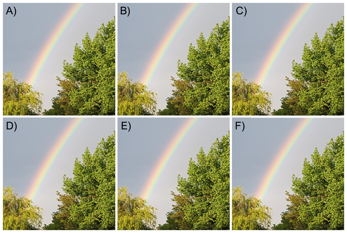
Figure 4: Visual comparison of a container image and corresponding stego images.
(A) Container color image. (B) Stego image with 100 chars embedded. (C) Stego image with 200 chars embedded. (D) Stego image with 300 chars embedded. (E) Stego image with 400 chars embedded. (F) Stego image with 500 chars embedded. The photos were taken by the authors.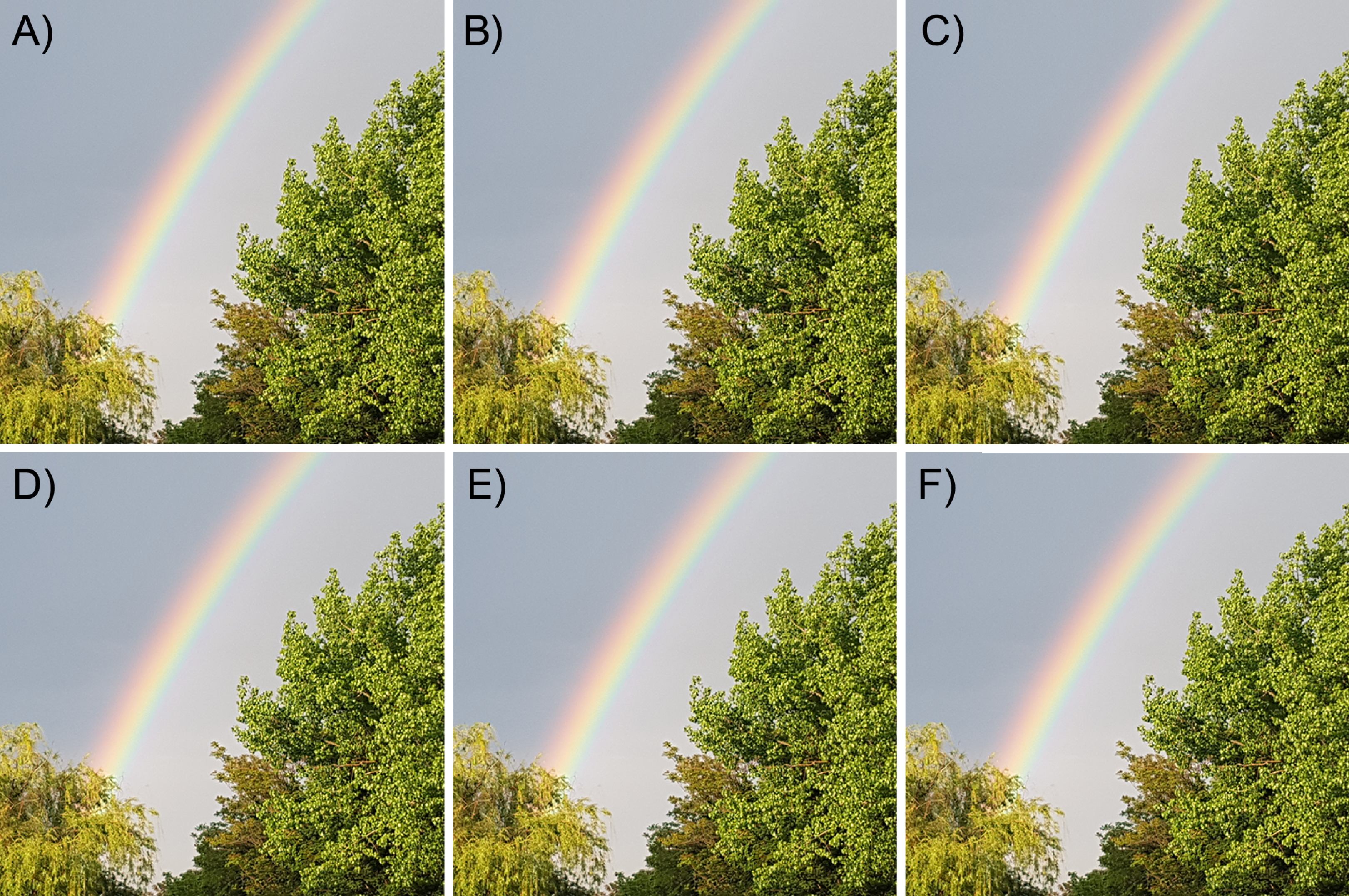
Figure 4 clearly demonstrates that there are no visual differences between the images and no traces of hidden messages. More examples are presented in Fig. 5, to confirm that there are no visual trace of steganography in corresponding stego images.
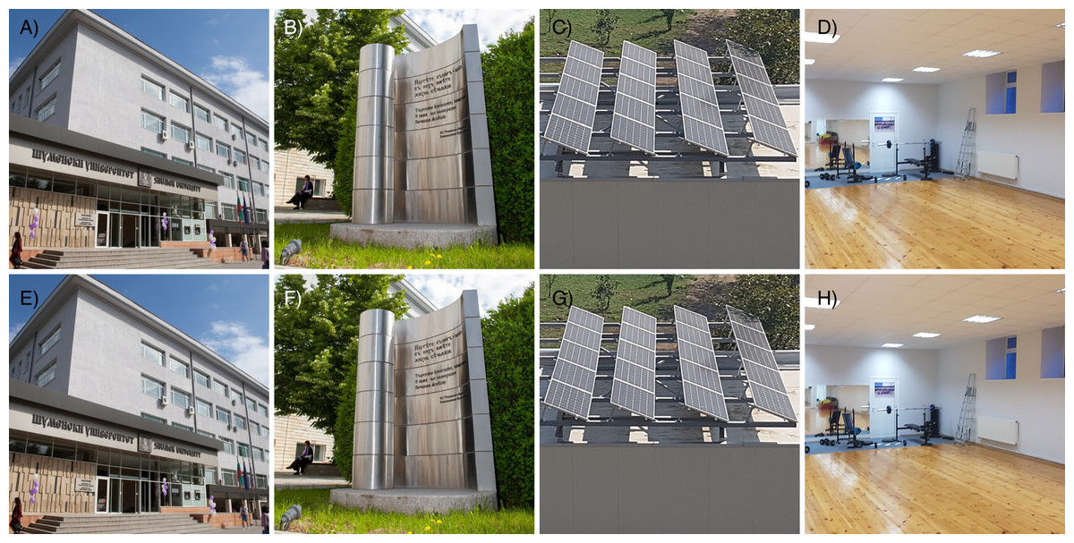
Figure 5: Additional examples of the proposed steganographic scheme.
(A) Container image—Main corpus. (B) Container image—Monument. (C) Container image—Solarpanels. (D) Container image—Fitness. (E) Stego image—Main corpus. (F) Stego image—Monument. (G) Stego image—Solar panels. (H) Stego image—Fitness. The photos were taken by the authors.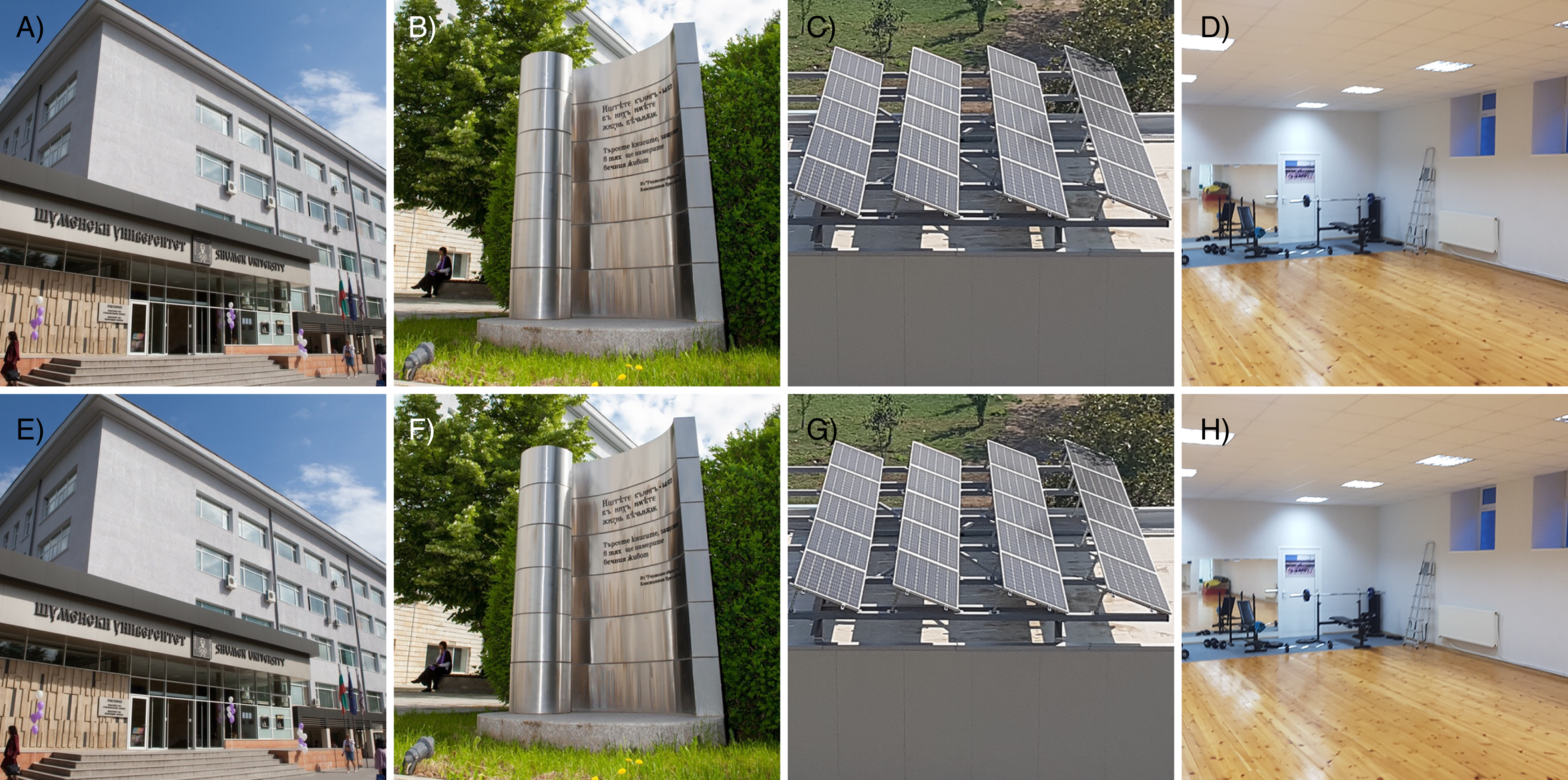
Histogram analysis
The image histograms are used for graphical representation of the tonal distribution of the red, green and blue colors. This experiment is designed to analyze if there are any changes in color distribution when the proposed steganographic method is applied.
Figure 6 shows the histograms of a test image with its corresponding stego images and Table 7 shows average pixel intensity values.
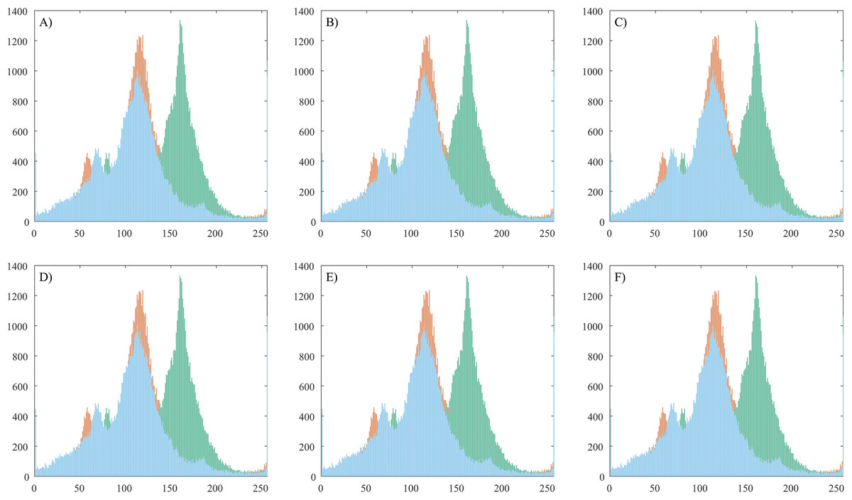
Figure 6: Histogram analysis of a plain image and corresponding stego images.
(A) Container color image. (B) Stego image with 100 chars embedded. (C) Stego image with 200 chars embedded. (D) Stego image with 300 chars embedded. (E) Stego image with 400 chars embedded. (F) Stego image with 500 chars embedded.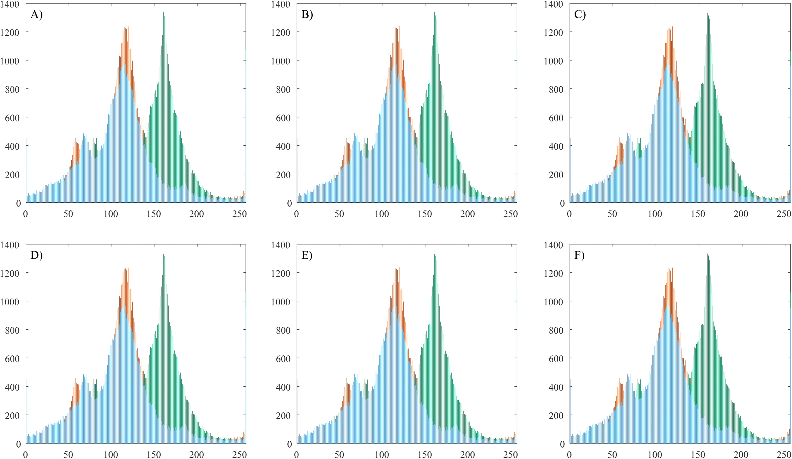
| File name | Plain Image Red | Stego Image Red | Plain Image Green | Stego Image Green | Plain Image Blue | Stego Image Blue |
|---|---|---|---|---|---|---|
| f1-256x256 | 157.731 | 159.385 | 130.011 | 157.731 | 159.385 | 130.010 |
| f2-256x256 | 152.790 | 127.875 | 102.467 | 152.790 | 127.875 | 102.466 |
| f3-256x256 | 127.915 | 129.950 | 134.474 | 127.915 | 129.950 | 134.473 |
| f4-256x256 | 111.816 | 115.017 | 86.290 | 111.816 | 115.017 | 86.290 |
| f5-256x256 | 173.490 | 159.482 | 142.303 | 173.490 | 159.482 | 142.302 |
| f6-256x256 | 114.214 | 114.245 | 111.757 | 114.214 | 114.245 | 111.757 |
| f7-256x256 | 111.514 | 141.846 | 107.249 | 111.514 | 141.846 | 107.249 |
| f8-256x256 | 120.503 | 117.243 | 108.933 | 120.503 | 117.243 | 108.933 |
| f1-512x512 | 157.678 | 159.365 | 129.554 | 157.678 | 159.365 | 129.554 |
| f2-512x512 | 152.831 | 127.877 | 102.465 | 152.831 | 127.877 | 102.465 |
| f3-512x512 | 127.888 | 129.910 | 134.402 | 127.888 | 129.910 | 134.402 |
| f4-512x512 | 111.793 | 115.004 | 86.060 | 111.793 | 115.004 | 86.060 |
| f5-512x512 | 173.511 | 159.513 | 142.351 | 173.511 | 159.513 | 142.351 |
| f6-512x512 | 114.465 | 114.475 | 111.955 | 114.465 | 114.475 | 111.954 |
| f7-512x512 | 111.546 | 141.904 | 107.253 | 111.546 | 141.904 | 107.253 |
| f8-512x512 | 120.562 | 117.298 | 108.986 | 120.562 | 117.298 | 108.986 |
The histogram attack method (Fridrich & Goljan, 2002) is historically the first statistical attack described in the resources. It is based on the fact that with LSB embedding, the even pixel values either remain unchanged (unmodified) or are being increased by 1, while the odd pixel values either remain unchanged or decrease. Thus, the values (2i, 2i + 1) form a pair of values (PoV), which are exchanged during embedding. This asymmetry in the embedding function can be used and a statistical test applied to confirm or deny that the even values follow the known distribution. The statistical steganalysis based on the Chi-square method is based on this. It makes a histogram (the frequency of occurrence of each color in the image) of the color distribution and based on it, pairs of adjacent values (PoV) are formed, differing in the youngest bit. Then a theoretical histogram of the color distribution is made, showing the expected distribution of the values in the presence of hidden information and pairs of adjacent values are formed again. The difference between the observed and expected occurrence frequencies for each pair is sought. In our case the observation of Fig. 6 shows that the tonal distribution is not changed when the secret messages are hidden in the plain image.
Peak signal-to-noise ratio and structural similarity analysis
The Peak Signal-to-Noise Ratio (PSNR) measure the possible maximum power of the clean signal against the power of the noise signal. Poorly changing the pixel values of an image can lead to corruption of the image quality which may uncover a possible steganography. PSNR is calculated using the following equation: (7) where MAX is the maximum possible value of the pixel color. Considering that every pixel has 8 bits for red, green and blue color, we use the average value of the three values meaning MAX = 28 − 1 = 255. MSE is the mean square error between the plain and stego images defined as: (8) where px,y and sx,y are the corresponding pixel values from the plain and stego images, respectively. Considering the color images have red, green and blue values for every pixel, the (px,y − sx,y)2 is calculated by: (9)
The Structural Similarity (SSIM) is another method used in steganographic analysis proposed and described in Wang et al. (2004). The test is designed to determine the similarity between two images, in our case the similarity between plain and corresponding stego images. Values close to 1 are indicators for the best possible structural similarity between the compared images.
Part of the obtained values for MSE, PSNR and SSIM are shown in Table 8. The MSE and PSNR values are calculated for images with 100 chars (800 bits), 1,000 chars (8,000 bits), and 2,000 chars (16,000 bits) embedded. All the results are available in Supplemental File 3.
| File name | Stego Image with 100 chars embbeded | Stego Image with 1,000 chars embbeded | Stego Image with 2,000 chars embbeded | ||||||
|---|---|---|---|---|---|---|---|---|---|
| MSE | PSNR | SSIM | MSE | PSNR | SSIM | MSE | PSNR | SSIM | |
| f1-256x256 | 0.001587 | 76.12527 | 0.999985 | 0.016464 | 65.96539 | 0.999859 | 0.032562 | 63.00366 | 0.999723 |
| f2-256x256 | 0.001480 | 76.42789 | 0.999986 | 0.015305 | 66.28259 | 0.999856 | 0.030289 | 63.31800 | 0.999715 |
| f3-256x256 | 0.001541 | 76.25239 | 0.999993 | 0.016159 | 66.04664 | 0.999917 | 0.031754 | 63.11288 | 0.999845 |
| f4-256x256 | 0.001511 | 76.33925 | 0.999996 | 0.015839 | 66.13363 | 0.999958 | 0.031494 | 63.14851 | 0.999921 |
| f5-256x256 | 0.001434 | 76.56432 | 0.999987 | 0.015823 | 66.13782 | 0.999865 | 0.031296 | 63.17595 | 0.999732 |
| f6-256x256 | 0.001556 | 76.20960 | 0.999992 | 0.015579 | 66.20535 | 0.999910 | 0.030823 | 63.24209 | 0.999825 |
| f7-256x256 | 0.001633 | 76.00177 | 0.999993 | 0.015717 | 66.16723 | 0.999929 | 0.030640 | 63.26797 | 0.999862 |
| f8-256x256 | 0.001526 | 76.29560 | 0.999993 | 0.015289 | 66.28693 | 0.999939 | 0.030563 | 63.27879 | 0.999878 |
| f1-512x512 | 0.000404 | 82.06314 | 0.999996 | 0.003708 | 72.43954 | 0.999969 | 0.007530 | 69.36273 | 0.999936 |
| f2-512x512 | 0.000366 | 82.49349 | 0.999996 | 0.003826 | 72.30319 | 0.999956 | 0.007805 | 69.20715 | 0.999910 |
| f3-512x512 | 0.000397 | 82.14587 | 0.999997 | 0.003601 | 72.56648 | 0.999975 | 0.007263 | 69.51953 | 0.999949 |
| f4-512x512 | 0.000408 | 82.02237 | 0.999998 | 0.003979 | 72.13336 | 0.999984 | 0.007813 | 69.20290 | 0.999969 |
| f5-512x512 | 0.000381 | 82.31620 | 0.999996 | 0.003731 | 72.41281 | 0.999960 | 0.007599 | 69.32331 | 0.999917 |
| f6-512x512 | 0.000347 | 82.72579 | 0.999998 | 0.003601 | 72.56648 | 0.999978 | 0.007313 | 69.48998 | 0.999955 |
| f7-512x512 | 0.000404 | 82.06314 | 0.999997 | 0.004047 | 72.05905 | 0.999968 | 0.008007 | 69.09608 | 0.999938 |
| f8-512x512 | 0.000370 | 82.44849 | 0.999998 | 0.003792 | 72.34234 | 0.999979 | 0.007710 | 69.26054 | 0.999958 |
Table 8 shows high values for PSNR (over 60 dB) meaning the stego algorithm do not destroy the image quality with considered minimum requirement of 20–30 dB for low quality. The obtained values for SSIM are close to the best possible value −1.
Additional metrics analysis
Some researchers use different metrics for steganographic analysis of their methods. For evaluation of the proposed algorithm we performed additional experiments for the most used indicators—Average Difference (AD), Structural Content (SC), Normalized Cross-Correlation (NCC), Maximum Difference (MD), Laplacian Mean Squared Error (LMSE), Normalized Absolute Error (NAE), Image Quality Index (IQI). The best possible value for SC, NCC, MD and IQI is 1 and for AD, LMSE and NAE is 0. The results for our method are presented in Table 8. All the results are available in Supplemental File 3.
The obtained results in Table 9 show results close to the perfect values demonstrating the stability and efficiency of the proposed stegoalgorithm.
| File name | AD | SC | NCC | MD | LMSE | NAE | IQI |
|---|---|---|---|---|---|---|---|
| f1-256x256 | 0.000061 | 1.00000 | 0.999999 | 1.000000 | 0.000003 | 0.000010 | 1.000000 |
| f2-256x256 | 0.000107 | 1.00000 | 1.000000 | 1.000000 | 0.000045 | 0.000011 | 1.000000 |
| f3-256x256 | 0.000015 | 1.00000 | 0.999999 | 1.000000 | 0.000009 | 0.000012 | 1.000000 |
| f4-256x256 | −0.000107 | 0.99999 | 1.000001 | 1.000000 | 0.000008 | 0.000014 | 1.000000 |
| f5-256x256 | −0.000122 | 0.99999 | 1.000001 | 1.000000 | 0.000029 | 0.000009 | 1.000000 |
| f6-256x256 | 0.000336 | 1.00000 | 0.999998 | 1.000000 | 0.000005 | 0.000014 | 1.000000 |
| f7-256x256 | 0.000076 | 1.00000 | 0.999999 | 1.000000 | 0.000026 | 0.000013 | 1.000000 |
| f8-256x256 | 0.000000 | 1.00000 | 1.000000 | 1.000000 | 0.000008 | 0.000013 | 1.000000 |
| f1-512x512 | 0.000000 | 1.00000 | 1.000000 | 1.000000 | 0.000001 | 0.000003 | 1.000000 |
| f2-512x512 | 0.000000 | 1.00000 | 1.000000 | 1.000000 | 0.000017 | 0.000003 | 1.000000 |
| f3-512x512 | 0.000023 | 1.00000 | 1.000000 | 1.000000 | 0.000004 | 0.000003 | 1.000000 |
| f4-512x512 | −0.000019 | 1.00000 | 1.000000 | 1.000000 | 0.000004 | 0.000004 | 1.000000 |
| f5-512x512 | 0.000008 | 1.00000 | 1.000000 | 1.000000 | 0.000024 | 0.000002 | 1.000000 |
| f6-512x512 | 0.000034 | 1.00000 | 1.000000 | 1.000000 | 0.000003 | 0.000003 | 1.000000 |
| f7-512x512 | 0.000038 | 1.00000 | 1.000000 | 1.000000 | 0.000078 | 0.000003 | 1.000000 |
| f8-512x512 | 0.000072 | 1.00000 | 0.999999 | 1.000000 | 0.000006 | 0.000003 | 1.000000 |
Comparison
In order to compare the proposed method with other image steganographic algorithms we use the presented metrics (where available) in related articles. The main metrics for defining the security and the reliability of the stegomethods are related to preserving the quality of the cover images and keeping the similarity with the stego images. For the image quality estimation the PSNR and MSE metrics are applied, and for the similarity of the cover and corresponding stego images—SSIM metric. The following Table 9 contains the most used metrics.
The test results in Table 10 show that the presented algorithm has satisfying statistical properties and provides better security level than compared methods.
| Reference | Average PSNR | Average MSE | Average SSIM |
|---|---|---|---|
| Proposed | 72.302898 | 0.007316938 | 0.999953563 |
| Chatterjee, Ghosal & Sarkar (2020) | 51.1070 | 0.4990 | 0.9981 |
| Yadav & Dutta (2017) | 65.0345 | 0.0374 | – |
| Amirulhaqi, Purboyo & Nugrahaeni (2017) | 66.3124 | 0.1473 | – |
| Baby et al. (2015) | 55.4522 | – | 0.7764 |
| Gaurav & Ghanekar (2018) | 47.8039 | 1.4468 | 0.9989 |
Chi-square analysis
In this article, steganalytic software based on the Chi-square method is used (available at http://www.guillermito2.net/stegano/tools/index.html). The software graphically shows the positions of the pixel values according to the image Chi-square value of the tested image. The red curve indicates the Chi-square values of the tested images and the green values represent the average value of the LSBs. If the green values are below the red curve the test didn’t pass successfully. Otherwise, it is assumed that the test was passed successfully, that is, there are no indications of a hidden message. For visual comparison we constructed a single screen shot image with six diagrams containing the results of the software.
Figure 7 demonstrates the results of our tests. The first is a diagram of the container and below are the corresponding stego files. The red curve is constantly at zero value leaving no green point under it. The Chi-square tests show that there is no trace of steganography in the stego files, indicated that the proposed algorithm can withstand against Chi-square attacks.
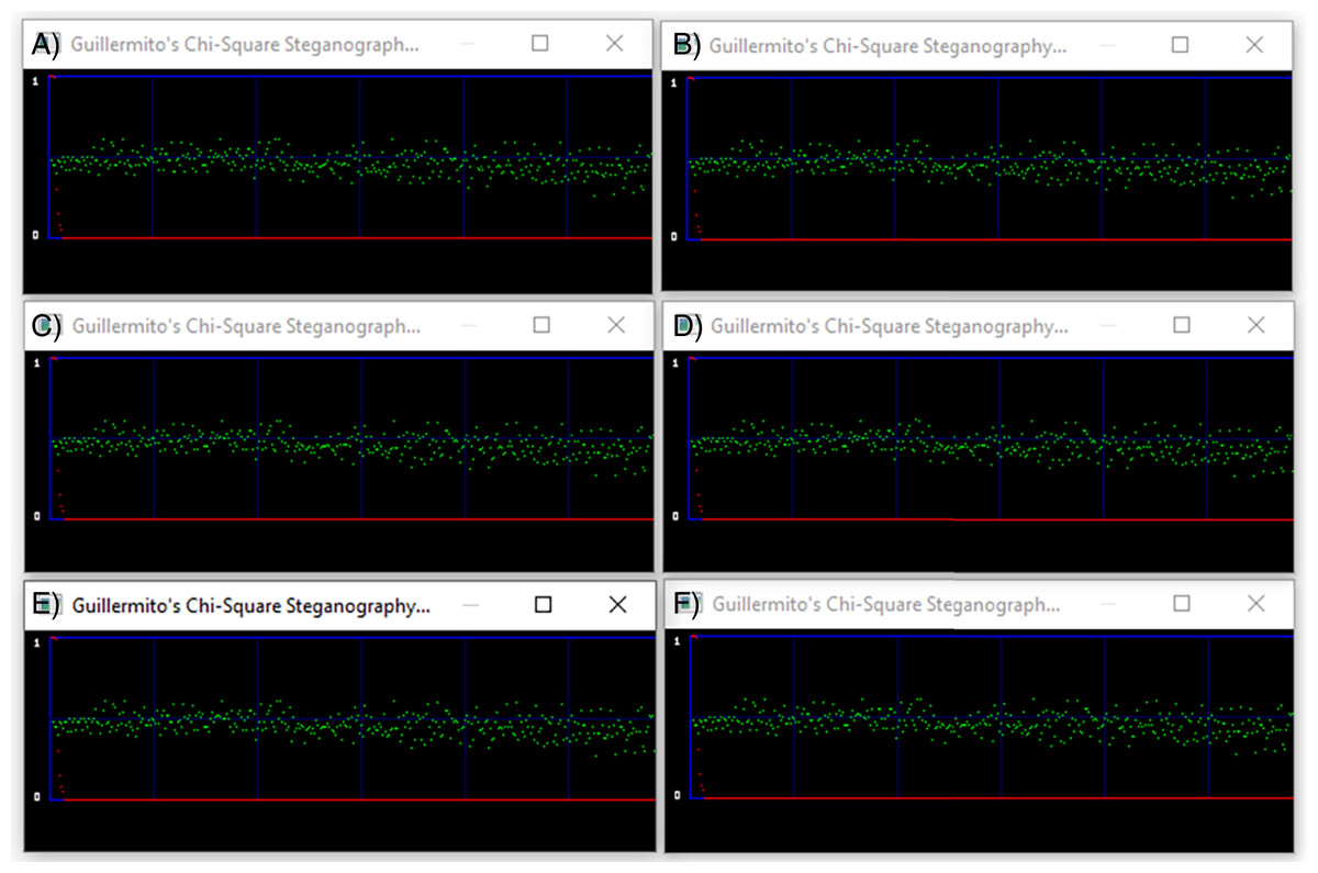
Figure 7: Chi-Square analysis of a container image and the corresponding stego images.
(A) Container color image. (B) Stego image with 100 chars embedded. (C) Stego image with 200 chars embedded. (D) Stego image with 300 chars embedded. (E) Stego image with 400 chars embedded. (F) Stego image with 500 chars embedded.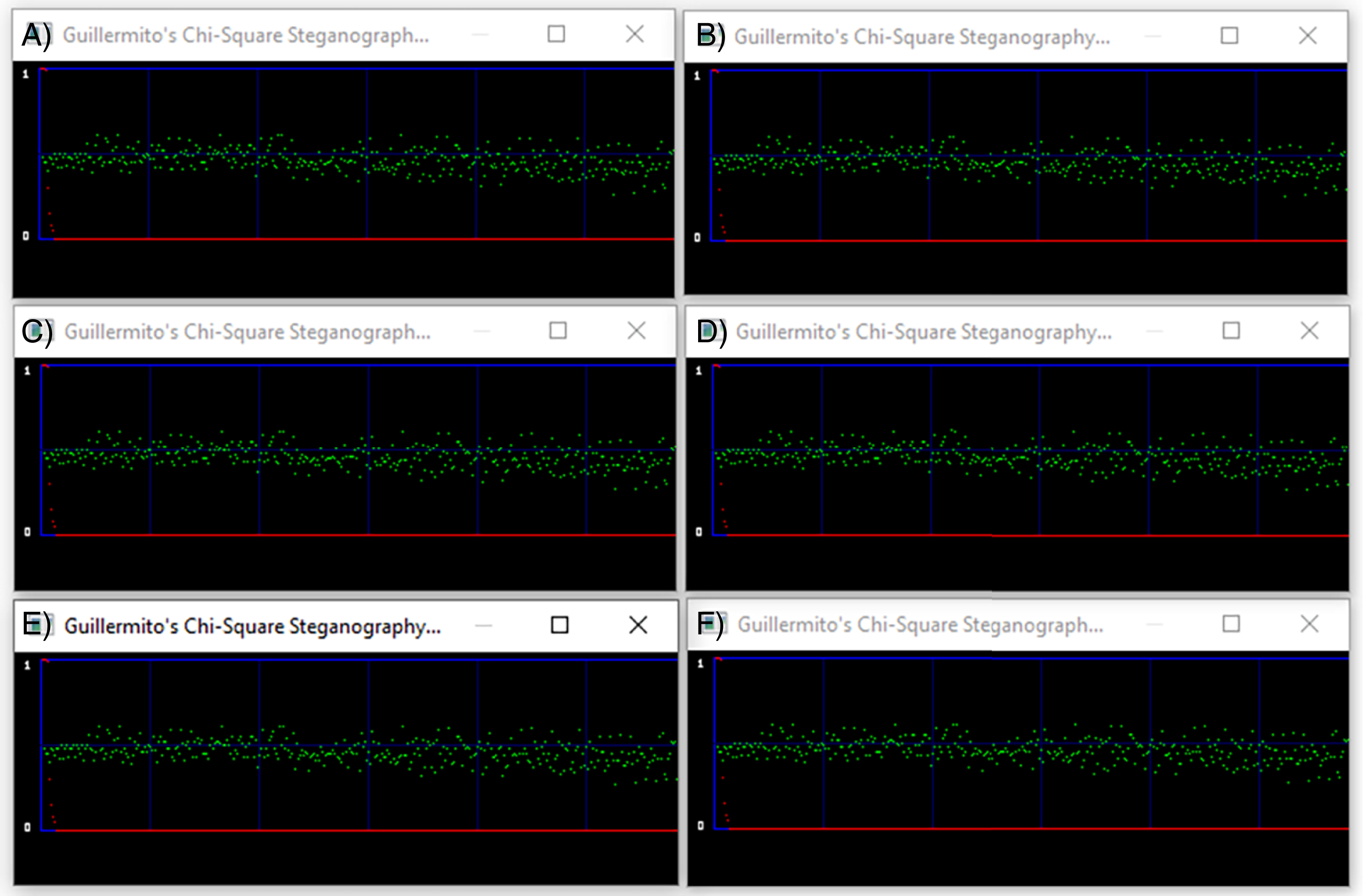
Computational and Complexity Analysis
The proposed algorithm is tested with the conditions described in Experimental Setup Section. Concerning the complexity of our method, it is defined by the computations and iterations of the calculations for encryption and embedding operations. Considering the linear computation of every operation(random numbers generation, LSB modification etc.) do not affect the complexity, the theoretical complexity of the proposed scheme is θ(8 * n) equated to θ(n), where n defines the input data of the algorithm. The input data of the algorithm is the secret message for embedding which is processed as bit sequence (8 bits for a character). The image parameters (width and height) do not increase the time consumption, because the number of random selected pixels depends only from the length of the embedded secret message. However, the images size is related to the memory consumption.
The following Table 11 summarizes the results of our empirical experiment for embedding different size of secret text messages.
| File name |
File dimensions |
Length of the secret message | ||||
|---|---|---|---|---|---|---|
| 100 chars | 500 chars | 1,000 chars | 1,500 chars | 2,000 chars | ||
| 800 bits (s) | 4,000 bits (s) | 8,000 bits (s) | 12,000 bits (s) | 16,000 bits (s) | ||
| f1-256x256.bmp | 256 × 256 | 0.001047 | 0.004402 | 0.008797 | 0.011602 | 0.016867 |
| f2-256x256.bmp | 256 × 256 | 0.000982 | 0.004679 | 0.009034 | 0.012969 | 0.017281 |
| f3-256x256.bmp | 256 × 256 | 0.001072 | 0.004439 | 0.009252 | 0.012871 | 0.017199 |
| f4-256x256.bmp | 256 × 256 | 0.001080 | 0.004546 | 0.008729 | 0.012998 | 0.017225 |
| f5-256x256.bmp | 256 × 256 | 0.001063 | 0.004473 | 0.008755 | 0.012997 | 0.017303 |
| f6-256x256.bmp | 256 × 256 | 0.001110 | 0.004423 | 0.008684 | 0.013166 | 0.016440 |
| f7-256x256.bmp | 256 × 256 | 0.001126 | 0.004425 | 0.009174 | 0.012913 | 0.017469 |
| f8-256x256.bmp | 256 × 256 | 0.001076 | 0.004401 | 0.008613 | 0.013002 | 0.016745 |
| f1-512x512.bmp | 512 × 512 | 0.001191 | 0.004556 | 0.008669 | 0.012760 | 0.017055 |
| f2-512x512.bmp | 512 × 512 | 0.001162 | 0.004795 | 0.008789 | 0.012951 | 0.017146 |
| f3-512x512.bmp | 512 × 512 | 0.001203 | 0.004614 | 0.008765 | 0.012883 | 0.017187 |
| f4-512x512.bmp | 512 × 512 | 0.001181 | 0.004670 | 0.009005 | 0.012835 | 0.017069 |
| f5-512x512.bmp | 512 × 512 | 0.000949 | 0.004530 | 0.009063 | 0.013088 | 0.016204 |
| f6-512x512.bmp | 512 × 512 | 0.001173 | 0.004571 | 0.008818 | 0.012261 | 0.017133 |
| f7-512x512.bmp | 512 × 512 | 0.001159 | 0.004522 | 0.008727 | 0.012643 | 0.017098 |
| f8-512x512.bmp | 512 × 512 | 0.001123 | 0.004362 | 0.008808 | 0.011896 | 0.017253 |
The results in Table 11 show that the proposed method is very fast and the computational complexity depends entirely of the secret text length.
Conclusions
In this manuscript a new method for steganography is presented. The base of the proposed algorithm is a PRG used for secret message encryption and random pixels selection for data embedding. Proving the level of security the PRG is statistically tested for randomness and key-sensitivity, and the key-space analysis defines a necessary level of brute-force attacks resistance with minimum requirement 2100 for key-space.
The steganographic algorithm is evaluated with visual analysis, file size comparison, histogram analysis and chi-square analysis and the results show that there are no traces of steganography when a secret message is hidden in the tested color images. The PSNR analysis indicates that the quality of the signal in stego images remains high, considered that the good quality of the signal is above 20 dB. Additional tests indicates high similarity between cover and the corresponding stego images for proving the security and the reliability of the proposed scheme. The presented method can be improved for real-time video communication with embedded data.
Supplemental Information
The first part of the test images.
Container images and stego images with 100, 200, 300 and 400 chars embedded. The photos were taken by the authors.
The second part of the test images.
Stego images with 500, 1000, 1500 and 2000 chars embedded.
Numerical data.
All the metrics of steganographic analysis.
The most important aspects of the source code.
The C++ code contains the Pseudorandom generator initial values and a function for extracting bits, the encryption and decryption code and bits embedding code.