
Elemental analysis by Metallobalance provides a complementary support layer over existing blood biochemistry panel-based cancer risk assessment
- Published
- Accepted
- Received
- Academic Editor
- Vladimir Uversky
- Subject Areas
- Biochemistry, Epidemiology, Hematology, Oncology
- Keywords
- Cancer biology, Chemical biology, Epidemiology, Mass spectrometry, Preventative medicine
- Copyright
- © 2021 Kusakabe et al.
- Licence
- This is an open access article distributed under the terms of the Creative Commons Attribution License, which permits using, remixing, and building upon the work non-commercially, as long as it is properly attributed. For attribution, the original author(s), title, publication source (PeerJ) and either DOI or URL of the article must be cited.
- Cite this article
- 2021. Elemental analysis by Metallobalance provides a complementary support layer over existing blood biochemistry panel-based cancer risk assessment. PeerJ 9:e12247 https://doi.org/10.7717/peerj.12247
Abstract
Despite the benefit of early cancer screening, Japan has one of the lowest cancer screening rates among developed countries, possibly due to there being a lack of “a good test” that can provide sufficient levels of test sensitivity and accuracy without a large price tag. As a number of essential and trace elements have been intimately connected to the oncogenesis of cancer, Metallobalance, a recent development in elemental analysis utilizing the technique of inductively coupled plasma mass spectrometry has been developed and tested as a robust method for arrayed cancer risk screening. We have conducted case-control epidemiological studies in the prefecture of Chiba, in the Greater Tokyo Area, and sought to determine both Metallobalance screening’s effectiveness for predicting pan-cancer outcomes, and whether the method is capable enough to replace the more conventional antigen-based testing methods. Results suggest that MB screening provides some means of classification potential among cancer and non-cancer cases, and may work well as a complementary method to traditional antigen-based tumor marker testing, even in situations where tumor markers alone cannot discernibly identify cancer from non-cancer cases.
Introduction
Despite being the leading cause of death since 1981 (Ministry of Health, Labour, and Welfare, Annual Vital Statistics Report Main Statistics, 2020), cancer, a number of types of which can be prevented with early screening and monitoring, often does not appear on most people’s radar until later in life. Japan, for instance, has one of the lowest cancer screening rates (Editorial Board of the Cancer Statistics in Japan & Cancer Statistics in Japan, 2021; OECD stat, 2020) in developed countries, yet only a few limited healthcare facilities are dedicated to screening and preventative medicine (Okuhara et al., 2018b). While multiplexed reasons, such as anti-cancer screening sentiments (Okuhara et al., 2018b), may have led to this current development, the lack of “a good test” is perhaps be the largest hurdle to clear to-date. In absence of such a test with sensitivity, reproducibility and low costs of entry, a bottleneck for the expansion rate for effective large-scale screening remains. Even as recent trends in biomedical advances have introduced to the public a barrage of modern instrumentation and testing such as genetic risk screening by next generation sequencing, or even methods that exploit a number of decided novel oncotargets such as MicroRNA, nucleosomes and even apoAII (PDQ Screening and Prevention Editorial Board, 2019; Sugimoto et al., 2010; Ito et al., 2015; Honda et al., 2015), the “bread and butter” of cancer screening remains the use of blood biochemistry panels (Fig. 1, purple) for common cancer antigens such as CEA, CA19-9, CA125, etc. (Hall et al., 2018), which are highly limited in the scope of coverage for screening cancer of various types.
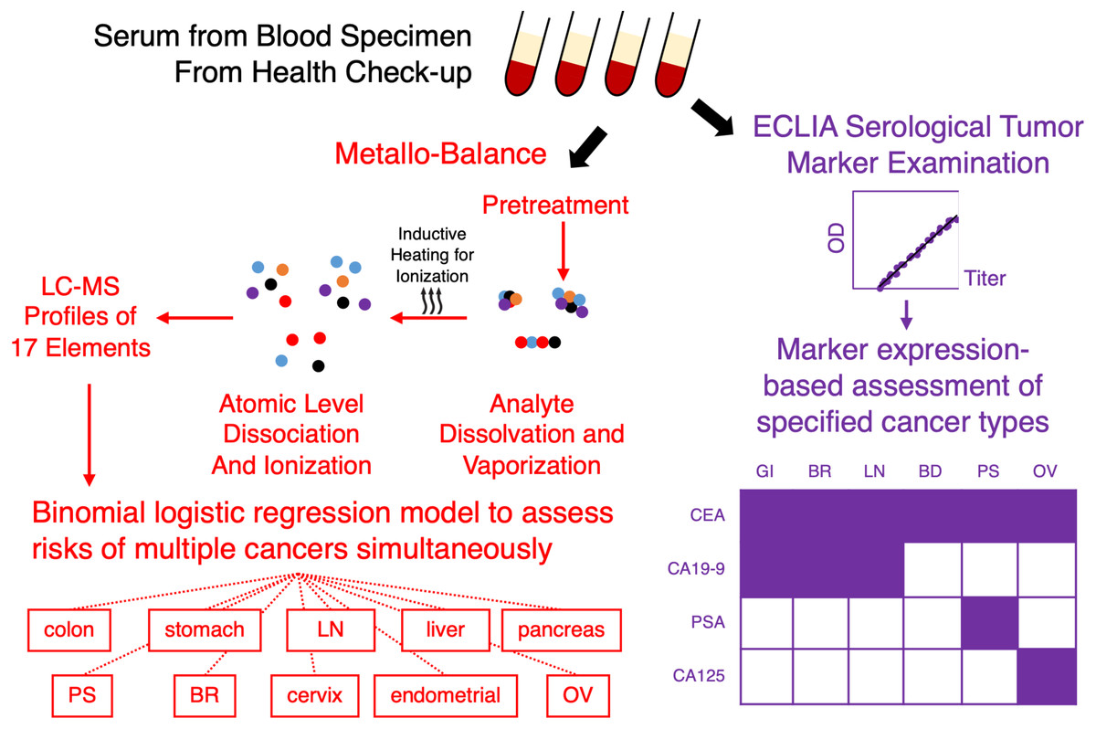
Figure 1: Metallobalance (MB) as a complementary test for pan-cancer screening.
Conventional serological examinations of tumor markers by methods such as electrochemiluminescence immunoassays (ECLIA), is only limited to a small known panel of markers, e.g., CEA, CA19-9, PSA and CA125; conversely, only a limited number of cancer susceptibility may be reportable (bottom right example; shaded grid indicates reportable type of cancer per marker; GI, gastrointestinal; BR, breast; LN, lung; BD, bladder; PS, prostate; OV, ovarian). Metallobalance (highlighted in red) on the other hand, utilizes induced collision plasma assisted mass spectrometric analysis to ionize serological analytes and produces a profile of 17 elemental levels. When combined cancer risk outcomes can generate logistic regression models to characterize susceptibility to a large number of cancer types simultaneously.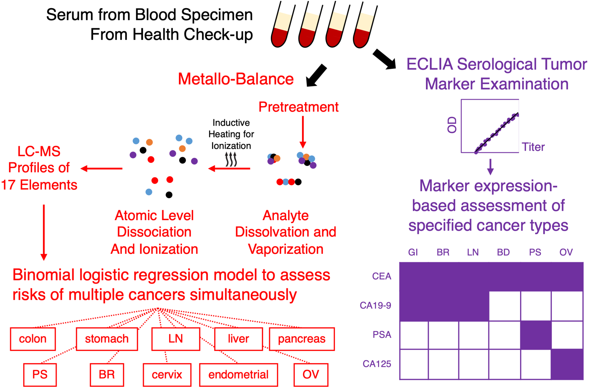
In analytical chemistry, elemental analysis is an essential tool for compound characterization; as elements not only compose the macromolecules that provide for life, their essential role in homeostasis and biological processes it is not difficult to make a natural connection for using elemental analysis to characterize human health and perhaps diseases such as cancer. Essential elements such as metals are intimately connected to carcinogenesis and metastasis; metalthioneine, for instance, is a protein involved in the regulation of metal ions, and has also been associated with tumor growth, differentiation and even drug resistance as others such as Manfei & Lang (2018) have investigated and concluded in a recent review. Additionally, interactions between metals such as Zn and Cu have also been said to cause dramatic effects on zinc-containing enzymes involved in processes leading up to cancer (Masoudreza et al., 2018). There is also association between serum elemental levels and cancer via events such as iron deficiency and oxidative stress, or baseline serum selenium levels with association to deaths from gastric cancer (Hu et al., 2018; Zhou et al., 2018).
A recent development in elemental analysis is Metallobalance (MB), an inductively coupled plasma mass spectrometry (ICP-MS)-based method to evaluate the comprehensive serum profile of 17 elements (Okamoto et al., 2020) for cancer screening (Fig. 1, red). A feature of MB is its ability to characterize, in addition to free elements in serum, elements in bound states such as the fundamental makeup of macromolecules. The test itself only requires small amounts of serum sample, can be stored and transported in absence of complex storage and protective measures, and thus can easily be implemented as part of the annual checkup procedure along with other tumor markers; additionally, the high-throughput nature and inexpensive preparation of ICP-MS also allows costs to be greatly reduced. On paper, however, while MB may be that one good test to promote large-scale screening, to-date MB only has risk prediction models for a handful of cancer types, partly due to an initial cohort of limited cancer type makeup. To characterize the applicability of MB as a pan-cancer screening tool, we have conducted case-control epidemiological studies in the prefecture of Chiba, in the Greater Tokyo Area, and sought to determine whether MB may be able to replace or supplement the more conventional antigen-based biomarker tests.
Materials & Methods
Study subjects
The ethics review committee at Chiba Cancer Center granted IRB approval (Cc# 902) for this study, and we obtained verbal informed consent from participants who later provided a signed consent form agreeing to specimen deposition at the Chiba Cancer Center Biobank. As part of a larger study, during the period of 2006 to 2013 we recruited and invited over 8,000 participants (M:F = 2,918:5,176) between the ages of 35 to 69 who resided in cities of Inzai, Abiko and Kashiwa in the prefecture of Chiba to participate in a cancer screening study which included blood specimen submission for multi-biomarker panel of CEA, CA 19-9, CA125 and PSA screening; remnants of the specimens were preserved and used for MB screening at a later time. In addition, these participants also volunteered responses to an epidemiological survey detailing their health histories and lifestyles, such as demographics, education, alcohol consumption, smoking, sleeping, exercise, food intake frequency, medication and supplement use, personal and family disease history, psychological stress, and female reproductive history. We selected those whose past medical histories had no indications of cancer as healthy individuals (cohort P0 henceforth; Table 1 left) based on records in the prefectural cancer registry kept and curated by the Cancer Prevention Center at Chiba Cancer Center.
| P0 | P1 | Excluded | |
|---|---|---|---|
| N | 5,327 | 1,856 | 1,491 |
| M: F | 1,696: 3,631 | 697: 1,159 | 544: 947 |
| Age [Mean] | 35∼69 [53.0] | 15∼94 [62.7] | 35∼69 [55.4] |
| <40 | 733 (13.8) | 106 (5.7) | 112 (7.5) |
| 40–49 | 1,332 (25.0) | 234 (12.6) | 315 (21.1) |
| 50–59 | 1,489 (28.0) | 257 (13.8) | 452 (30.3) |
| 60–69 | 1,773 (33.2) | 623 (33.6) | 612 (41.1) |
| >69 | 0 | 636 (34.3) | 0 |
| CEA | 2,090 | 1,331 | 258 |
| CA19-9 | 2,795 | 980 | 683 |
| CA125 | 2,003 | 521 | 435 |
| PSA | 748 | 231 | 184 |
Notes:
P0, non-cancer individuals; P1, cancer subjects; N, number of subjects within cohort; M:F, male:female ratio; Age, age range with estimated mean within bracket; value inside parentheses for individual age groups indicate percent of the subjects within cohort.
For the cohort of cancer cases P1 (Table 1 center) we selected a cohort of patients who visited our medical center for inpatient or outpatient services from 2013 to 2019, and consented to a biobank deposit of blood specimens for the study. P1 subjects all received diagnoses of cancer at our center and provided informed consent for the study. Cancer types among P1 subjects included cancers of the colon and rectum (N = 100, M:F = 60:40), stomach (N = 90, M:F = 150:68), liver (N = 117, M:F = 89:28), bile duct (N = 45, M:F = 22:68), pancreas (N = 233, M:W = 112:121), thyroid (N = 90, M:F = 34:56), prostate (N = 200), breast (N = 322), ovary (N = 79), cervix (N = 197), and uterine body (N = 148), and from their medical histories we recorded gender, age as well as cancer history; while some in P0 self-reported history of cancer, those (“Excluded” in Table 1) were excluded from subsequent analysis. In the case of P1 subjects who had more than one biomarker reading as a result of multiple visits to our hospital, we used the median value as the representative biomarker level.
Metallobalance screening by ICP-MS
After specimen collection, the operation of ICP-MS for MB screening was performed by Renatech Corporation (Isehara, Kanagawa, Japan), following the procedure for sample pretreatment and spectrometric analysis by inductively coupled plasma mass spectrometry as previously described in Okamoto et al. (2020). Briefly, 50 µl of serum samples were washed with ultra-pure water and 10% nitric acid along with cycles of heating for digestion; analytes were then treated with 61% nitric acid (v/v HNO3: analyte = 2.5:1) and 30% hydrogen peroxide (v/v 0.5:1) for 16 h at 70 °C in preparation for in-line plasma ionization and mass spectrometric characterization. The 17 different elemental levels acquired on a Agilent 7800 ICP-MS system under high-frequency output mode (1550 W) were as follows: Na (ppm), Mg (ppm), P (ppm), S (ppm), K (ppm), Ca (ppm), Fe (ppb), Co (ppb), Cu (ppb), Zn (ppb), As (ppb), Se (ppb), Rb (ppb), Sr (ppb), Mo (ppb), Ag (ppb) and Cs (ppb) against an internal standard of 50 µg/L beryllium, 5 µg/L yttrium, 1 µg/L rhodium and 50 µg/L tellurium at flow rates of 15 L/min and 1.05 L/min for plasma and nebulizer gases.
Data analysis
Statistical analysis was performed in R (ver. 4.1) with packages ggplot2 (ver. 3.3.3), effsize (ver. 0.8.1), caret (ver. 6.0.86), umap (ver. 0.2.6.0), RColorBrewer (ver. 1.1.2), smotefamily (ver. 1.3.1), pROC and gplots (ver. 3.0.4) (Wickham, 2020; Marco, 2020; Kuhn et al., 2008; Siriseriwan, 2019; Robin et al., 2011). Logistic regression models of the outcome of cancer history from MB elemental levels were generated to determine the odds ratio for individual elements. Due to the relative imbalance in population size, oversampling by SMOTE with 5 nearest neighbors was performed; results reported herein were averages over 1000 randomized samplings. Random forest classifier models associating MB levels with cancer history were trained on resultant SMOTE datasets with a 10% holdout and 500 trees; receiver operating characteristics were calculated from out of bag classification votes for each data point. Exploratory analysis via UMAP was performed using data obtained from MB for cohorts P0 and P1 after a parameter search for the number of nearest neighbors from 5 to 20 (final 5). Effect size comparisons were performed after log-transformation of MB data and subgroup stratification by gender and cohort; Cohen’s d score was then determined per cancer type via comparison to P0, where d > 0 indicated that there existed some measurable level of difference between the two cohort means, as normalized by the standard deviation of each respective elemental level. Generalized Gaussian linear regression models with identity link functions were used to create association models between elements included in the MB panel with common tumor markers. MB elemental levels were min-max scaled, while tumor biomarker levels were either log- (CA19-9, CA125, PSA) or square-root-transformed (CEA). For regression model building, CA19-9 readings beyond the cut-off of 2.0 U/ml were excluded as a precaution to ensure data quality. Reference “normal” thresholds of CEA < 5.0 ng/mL, CA19-9 < 37.0 U/mL, CA 125 < 35.0 U/mL and PSA < 4.0 ng/mL were established from a literature survey (Bast et al., 1983; Coric et al., 2015; Scara, Bottoni & Scatena, 2015; Konishi et al., 2018a), in line with cutoffs used in typical clinical serological examinations. A predefined alpha level of p < 0.05 was used for significance comparison, unless otherwise specified. Multiple comparison adjustments were not explicitly considered due to the exploratory nature of this study, however as a precaution for overfitting we adopted the alpha level of p < 0.0001 for regression models to account for cohort sizes.
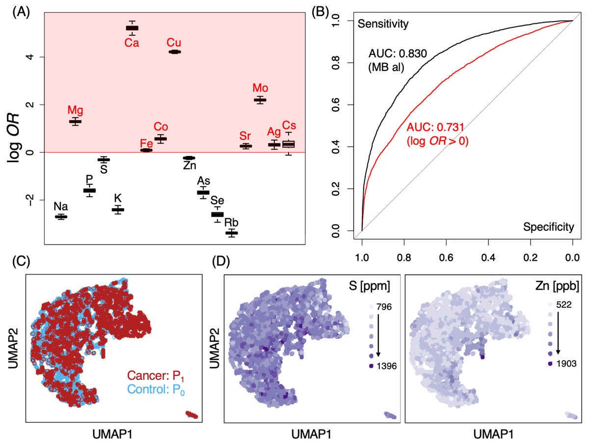
Figure 2: ICP-MS levels of certain elements may provide well differentiable indicators for cancer occurrence.
(A) log odds-ratios (OR) of elements tested in MB screening. Red shaded regions indicate those with log OR > 0 for cancer occurrence; results shown of average ORs from 1000 random SMOTE sampling trials. (B) ROC analysis of MB logistic regression classifier models for P0 and P1; black, all elements; red, model constructed only from those with log10OR >0; AUC, area under curve. (C, D) Distributional overlap of study cohorts by UMAP. Labeled colors indicate various conditions, either by cohort population (C) or by elemental levels (D). S (left) and Zn (right) are shown for representative purposes, gradients of light to dark purple indicate low to high elemental levels;P0, non-cancer control; P1, cancer cases.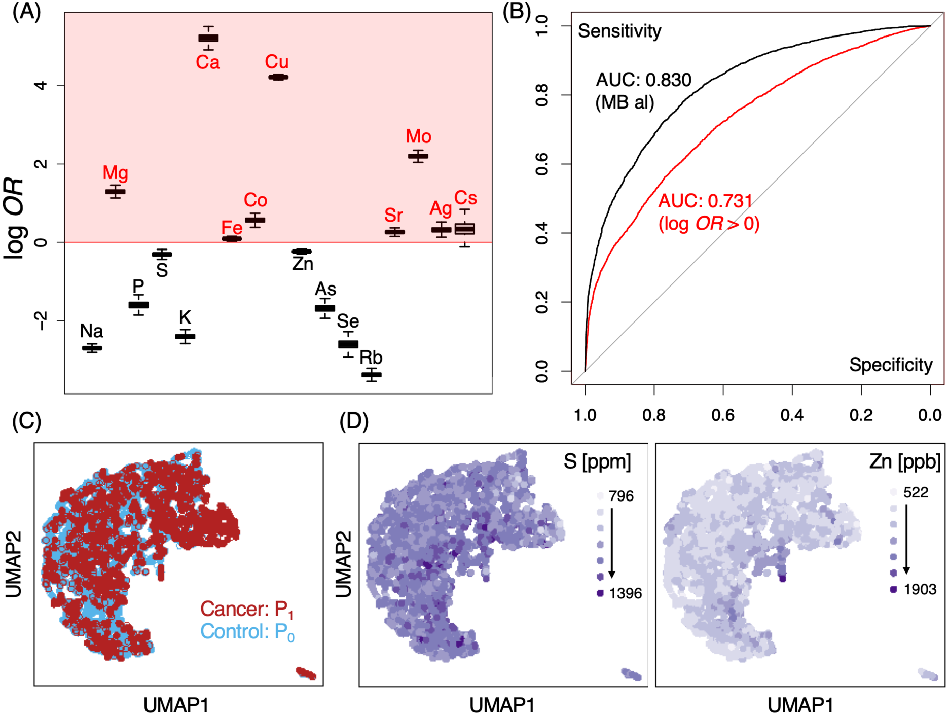
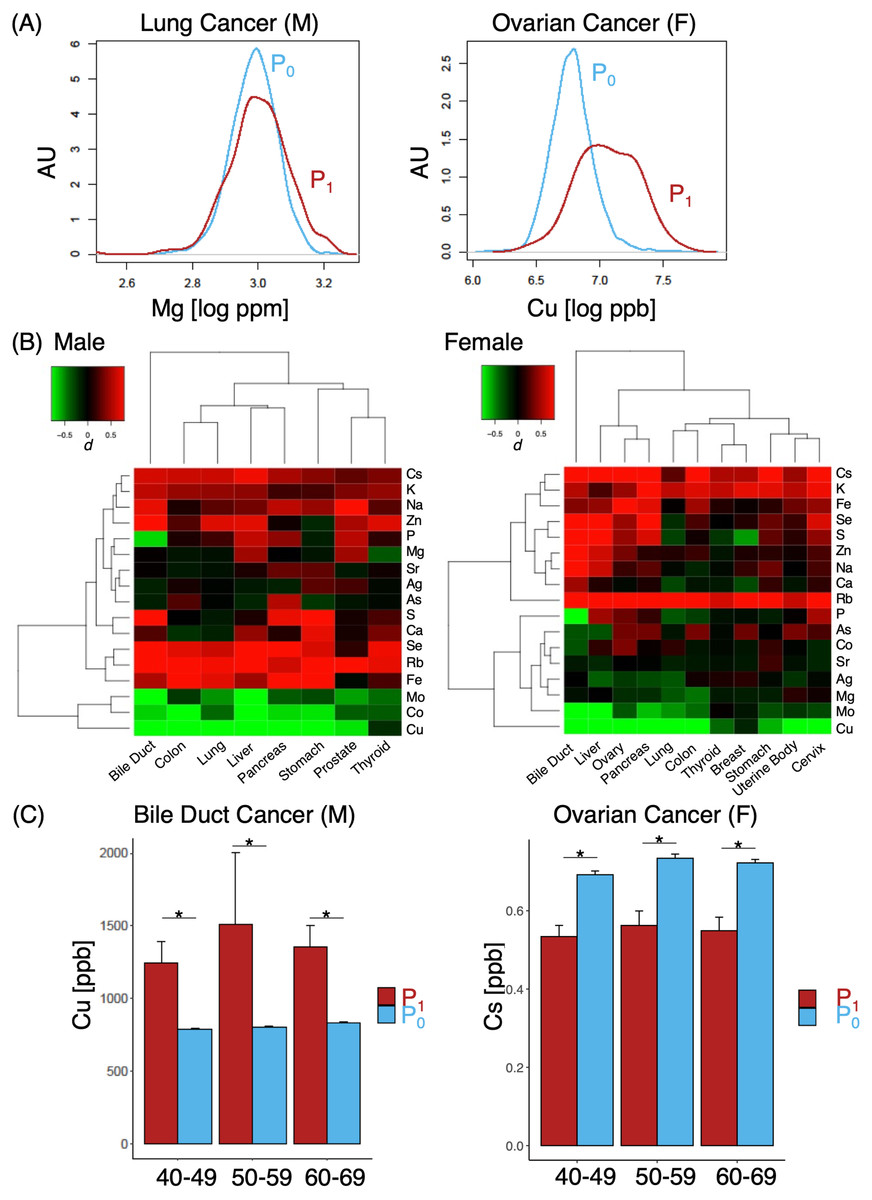
Figure 3: Differences in effect size in MB profiles.
(A) Representative cases of elements with small (lung cancer, left) and large (ovarian cancer, right); (B) heat map of various different cases and corresponding effect sizes of P1, with color gradients of d indicated in the upper left corner; (C) comparison of Cu (left) and Cs (right) levels between P0 and P1 cohorts. M, male; F, females. Asterisk, p < 0.05.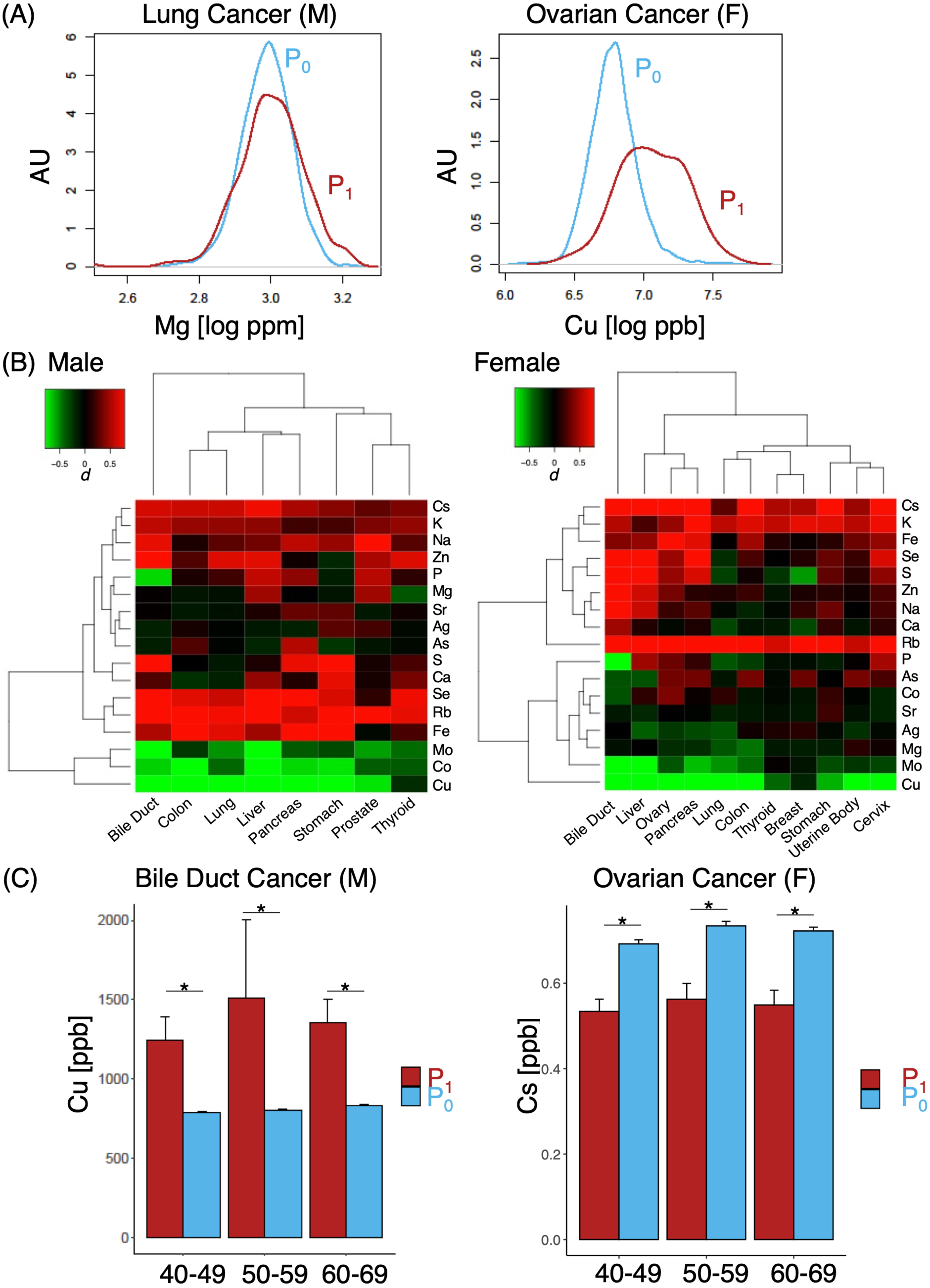
Results
A number of elements such as Mg, Ca, Fe, Co, Cu, Sr, Mo, Ag and Cs demonstrated some likelihoods of in their ability to discern cancer from non-cancer cases (Fig. 2A, log OR > 0). Pan-cancer logistic regression models (Fig. 2B) suggested cancer cases could be sufficiently identified from P0 at an AUC of 0.830 (0.731 when only elements with log OR > 0 were used). At the same time, however, we also observed a large portion of overlap in P0 and P1 MB profiles in two-dimensional UMAP (Fig. 2C) and poorly defined separation boundaries; while certain gradients in elemental levels existed (Fig. 2D), straight-forward identification of cancer (P1) from healthy subjects (P0) was not trivial, indicating that data collection might be insufficient with a cohort of this size. To evaluate whether the overlap also occurred at the individual elemental level, we examined the effect size distributions via Cohen’s d for each element among different cancer types in comparison to P0 (Fig.3A; Fig. S1). Cohen’s d provided a metric to highlight the distributional differences by standardized means free from influences of sample size, a feature in which the cancer cases are typically dwarfed by the size of the control cohort. We qualitatively evaluated effect sizes (Table 2) using the following boundaries: a difference of —d— < 0.2 was considered negligible, while values lower than 0.5, 0.8 and those above 0.8 were evaluated as small, medium and large differences, respectively. Effect sizes were also determined along gender lines, with men exhibiting a range of −3.25 to 1.70 and women from −2.5 to 1.77 (Fig. 3B). Elements found to have an odds ratio of log OR > 0 also exhibited statistically significant differences across various cancers, for instance Cu in bile duct cancer in men and Cs in ovarian cancer for women (Fig. 3C). Effect sizes were markedly different among different cancer sites, suggesting that a comparison of multiplexed elemental levels had the potential for cancer risk evaluation. Several elements in P1 had large effect sizes in a number of cancers (Table 3) in men, while a slightly different pattern was observed in women (Table 4). Comparisons of elemental levels in various age-matched groups (40–49, 50–59, 60–69; Table 5) revealed that a handful of elements appeared to have less overlap in the younger subpopulations in the two cohorts. As a whole, serum elements exhibited enough differences in their distribution as evidence of indicator effectiveness for characterizing cancer risks.
| Stomach | Liver | Thyroid | Colon/Rectum | Bile duct | Lung | Pancreas | |
|---|---|---|---|---|---|---|---|
| dlow | −0.72 | −1.54 | −0.29 | −0.01 | −2.64 | −1.22 | −1.80 |
| dhigh | 1.24 | 1.10 | 0.66 | 0.93 | 1.37 | 0.75 | 0.99 |
Notes:
dlow, minimum Cohens d observed; dhigh, maximum Cohens d observed.
| Element | Stomach | Liver | Prostate | Colon | Bile duct | Lung | Pancreas |
|---|---|---|---|---|---|---|---|
| S | 1.36 | 0.85 | |||||
| Fe | 1.10 | 1.03 | 1.06 | ||||
| Cu | −1.04 | −1.86 | −1.19 | −3.25 | −1.66 | −2.18 | |
| Rb | 0.97 | 1.13 | 0.81 | 0.82 | 1.23 | ||
| Se | 1.33 | 1.70 | 1.22 | ||||
| Mo | −0.94 | 0.85 | |||||
| Na | 0.81 | ||||||
| Co | 1.14 | −1.37 |
| Element | Ovary | Liver | Pancreas | Colon | Bile duct |
|---|---|---|---|---|---|
| S | 1.38 | ||||
| Fe | 0.88 | ||||
| Cu | −1.65 | −1.90 | −1.75 | −1.31 | −2.50 |
| Rb | 1.01 | 1.15 | 1.37 | 1.17 | 1.77 |
| Se | 1.01 | 0.94 | 1.37 | ||
| Mo | −1.12 | −0.9 | |||
| Na | 1.07 | ||||
| P | −2.51 | ||||
| K | 0.86 | ||||
| Cs | 0.95 | 0.81 | 0.96 | 0.91 | 1.12 |
| Sex | Cancer site | Element | Age group | P1/P0 (p-value) |
|---|---|---|---|---|
| M | Prostate | Na[ppm] | 40–49 | 3171/3227 (0.02) |
| 50–59 | 3170/3228 (<0.001) | |||
| 60–69 | 3264/3232 (<0.001) | |||
| K[ppm] | 40–49 | 164/169 (0.0192) | ||
| 50–59 | 160/168 (0.0496) | |||
| 60–69 | 165/172 (<0.001) | |||
| Rb[ppb] | 40–49 | 180/177 (0.0004) | ||
| 50–59 | 158/167 (0.0046) | |||
| 60–69 | 149/165 (<0.001) | |||
| Bile duct | Cu[ppb] | 40–49 | 1245/793 (0.0229) | |
| 50–59 | 1512/808 (0.0219) | |||
| 60–69 | 1357/834 (0.0136) | |||
| Pancreatic | Cu[ppb] | 40–49 | 1341/793 (0.01769) | |
| 50–59 | 1319/808 (0.0017) | |||
| 60–69 | 1223/834 (<0.001) | |||
| F | Ovarian | Rb[ppb] | 40–49 | 151.3/172.4 (0.014) |
| 50–59 | 147.6/164.8 (0.019) | |||
| 60–69 | 131.6/158.8 (0.035) | |||
| Cs[ppb] | 40–49 | 0.53/0.69 (0.013) | ||
| 50–59 | 0.56/0.73 (<0.001) | |||
| 60–69 | 0.55/0.72 (<0.001) | |||
| Uterine body | K[ppm] | 40–49 | 159.4/166.2 (0.0166) | |
| 50–59 | 157.4/165.5 (0.017) | |||
| 60–69 | 160.8/168.0 (<0.001) | |||
| Cervical | K[ppm] | 40–49 | 156.6/166.2 (0.028) | |
| 50–59 | 155.1/165.5 (0.037) | |||
| 60–69 | 152.4/168.0 (<0.001) | |||
| Se[ppb] | 40–49 | 134.3/138.6 (0.079) | ||
| 50–59 | 132.6/144.5 (<0.001) | |||
| 60–69 | 134.0/145.6 (0.002) |
Tumor markers such as CEA, CA19-9, CA125, PSA were routinely measured for cancer risk screening during annual health checkups, and while these were reasonable indicators on some level, we found that there was a great overlap in marker levels deemed normal in both P0 and P1 cohorts (Table 6); essentially, tumor markers alone could not sufficiently differentiate the two cohorts (Fig. 4), hinting that a limited serological panel of tumor markers were insufficient for cancer risk assessment. To validate MB’s performance as a supplemental tool for risk assessment, we created 2 generalized linear regression models, to identify potential associations, using MB profiles to compare correlations between marker expression in these two cohorts. A number of elements appeared to have more distinguished influences in model performance in the cancer cohort (Fig. 5A); for those identified with normal values of CEA, elements such as Na, K, Cu, Fe Co and Mo exhibited visible differences in mean in P1 over the non-cancer P0 cohort; similarly, Zn, Cs, Ag, and Mo appeared to be significantly different in mean for normal CA19-9 readings, while for CA125 P, As, Cu, Fe, Mo and Cs and for PSA K, Zn, Rb, Mo and Cs (Fig. 5B), notably intersecting with our earlier observations in Fig. 2A. Someone with a normal tumor biomarker reading, for instance, could potentially benefit from a supplemental MB screening for abnormal levels of elements such as Cu, Mo, Ag and Cs as support indicators for cancer risks.
| Marker | P0 | P1 |
|---|---|---|
| CEA | 2,015 | 1,147 |
| CA 19-9 | 2,367 | 747 |
| CA125 | 1,949 | 456 |
| PSA | 714 | 208 |
Notes:
N0 = 5,327; N1 = 1,856.
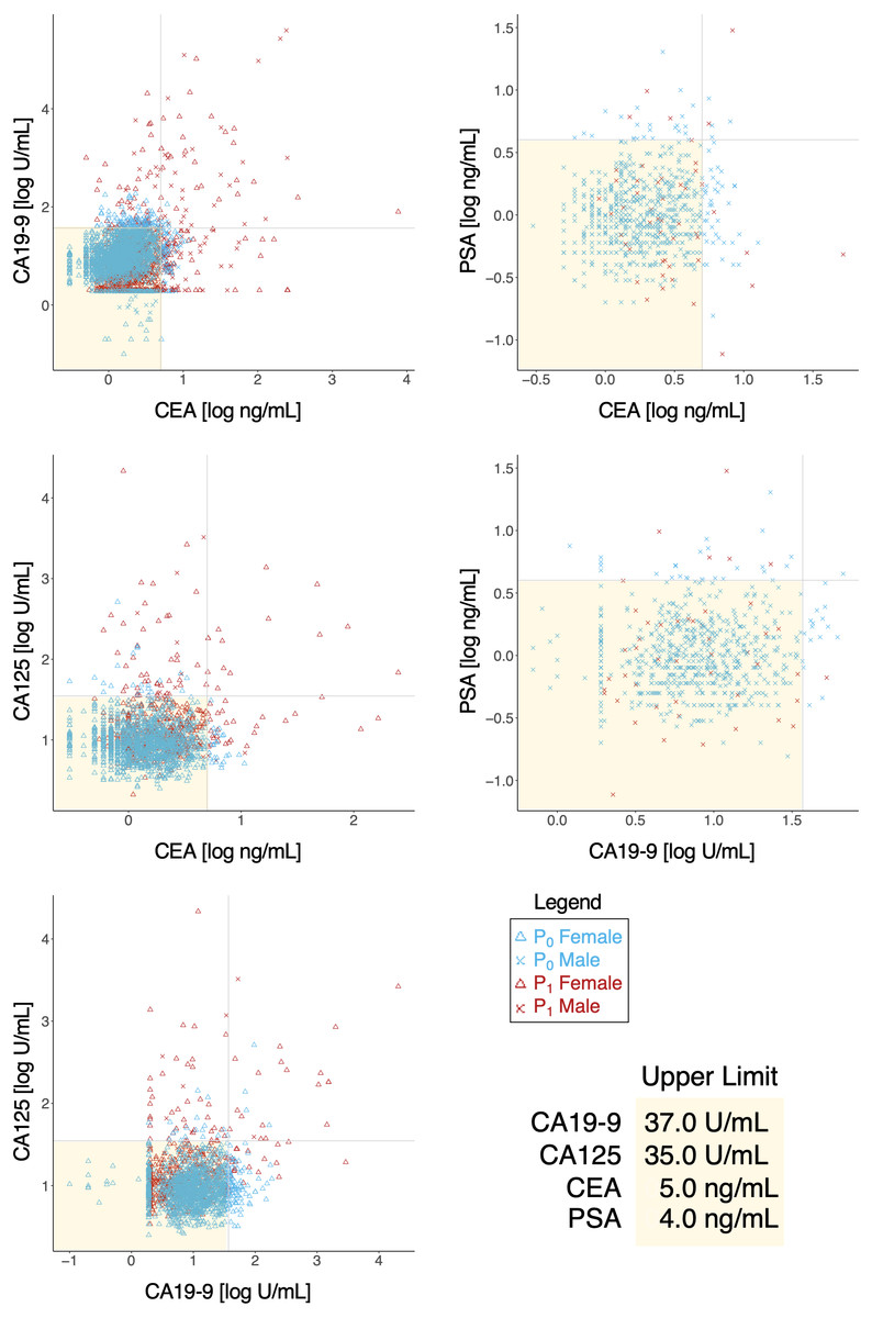
Figure 4: Behavior of tumor biomarkers in cancer and non-cancer cases.
Shaded yellow region indicates normal thresholds (upper limit, bottom right) for each respective marker. Vertical and horizontal axes indicate pairings of tumor biomarkers and concentration.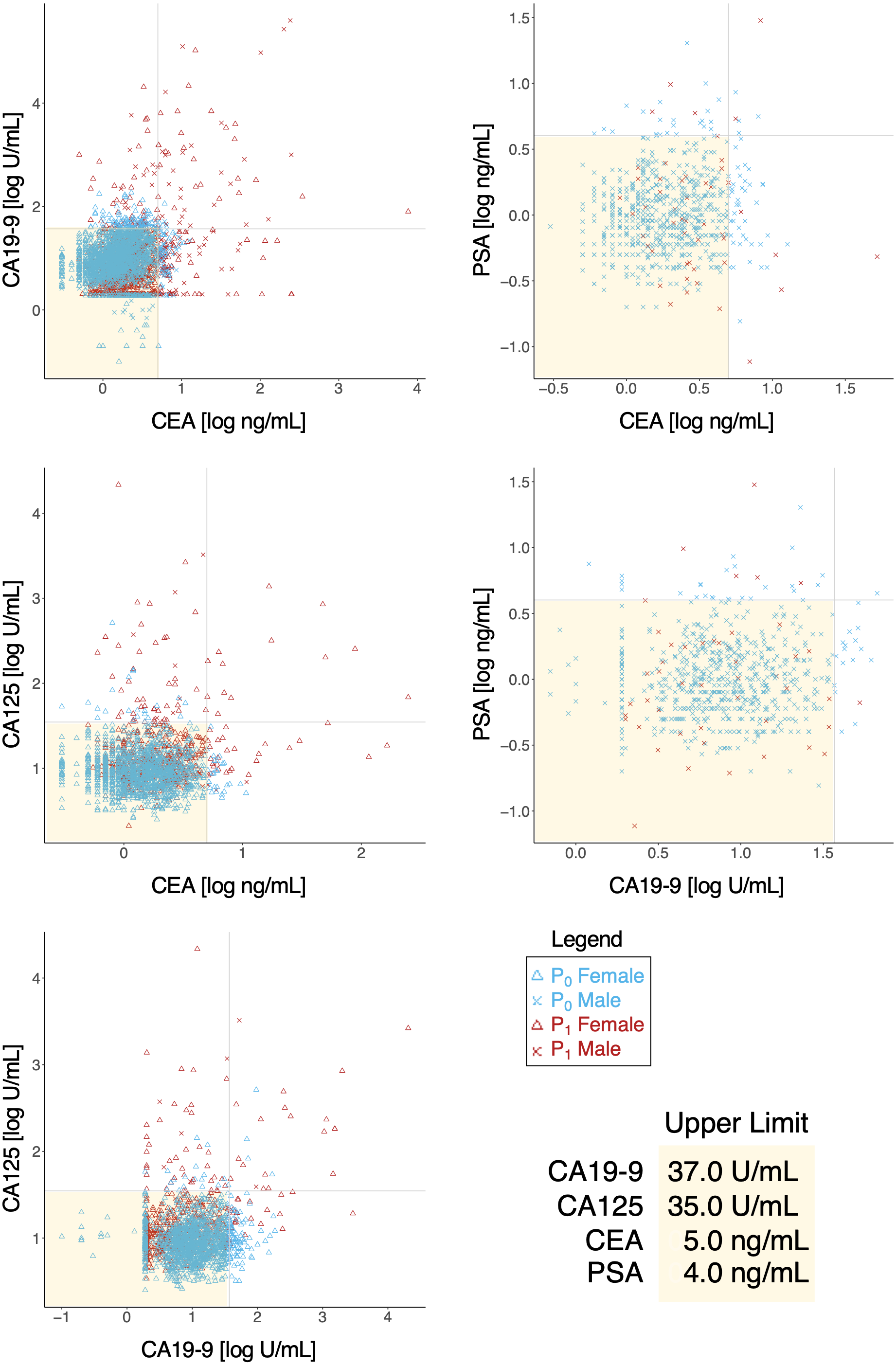
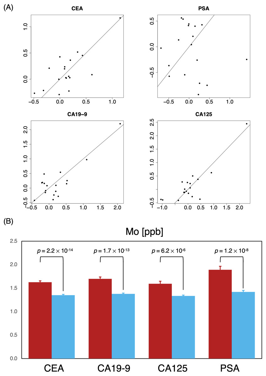
Figure 5: Identifying critical elements as support indicators for tumor biomarkers.
(A) Two-dimensional comparison of generalized linear regression coefficients non-cancer (P0, horizontal axes) vs. cancer (P0, vertical axes) of MB elements; solid reference line has a slope of 1. (B) Comparison of mean Mo levels among subjects with normal marker ranges; P0 red; P0, blue.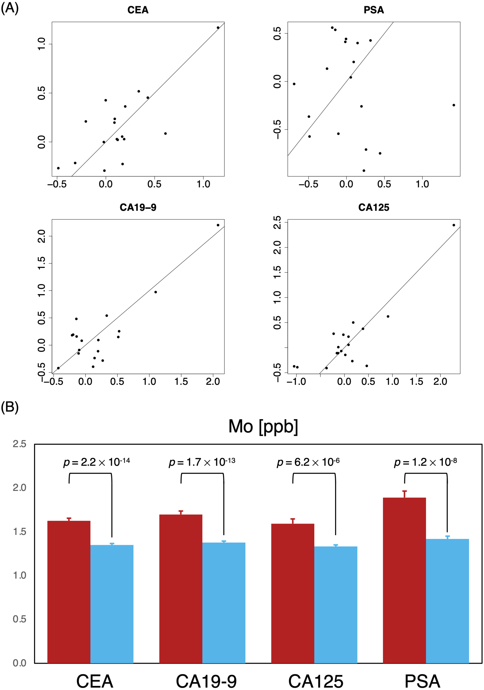
Discussion
While observations here largely affirmed some of our previous findings (Okamoto et al., 2020), a direct multivariate analysis of neither biomarker levels nor MB results alone curiously provided sufficient degrees of separation between the cancer and non-cancer cohorts surveyed with ∼7,200 participants. There were nonetheless elements with abundance differences indicative of statistical significance, when grouped together or otherwise as seen in Fig. 2A. In consideration of some of the associations to cancer outcome as seen in Fig. 2, the use of MB should be able to supplement more conventional serological exams for a number of cancer types simultaneously. These odds ratios also provide a way to aggregate results statistically (e.g., via geometric mean) from a cluster of elements to assess against reference values in a similar manner marker expression or activity levels provide. This is perhaps also advantageous for result interpretation, since the new aggregated scores can be normalized for different populations, and similarly monitored by tracing trends in the rate of changes in score over time.
Gender differences also existed to some extent, although it was not as pronounced as we expected; additionally, element with significantly different abundances across cohorts were also seen in groups where expressions of commonly used tumor markers failed to discern cancer from non-cancer individuals. While serum elemental levels had been implicated in estimating risks of susceptibility for a handful of cancers (Okamoto et al., 2020), it was perhaps, whilst erring on the side of conservatism, fitting to conclude that a comprehensive elemental profile would see better performance alongside tumor marker levels in a serological examination. An ICP-MS based elemental analysis method, when performed as a companion screening test to the usual tumor marker panels, could potentially improve the sensitivity and specificity of existing cancer screening methods. As an additional screening, it could potentially help physicians make decisions about whether a follow-up and more invasive or costly method of screening, i.e., colonoscopy or gastroendoscopy, would be necessary for someone who had an above-normal CEA reading (Lennon et al., 2020). Element with large effect sizes were particularly effective in distinguishing cancer from non-cancer subjects, for example in the case of cancers of the bile duct and liver in both men and women. For Cs, we found that the effect size was exclusively elevated in women, leading us to posit that gender-specific risk models could be a necessity in future investigations or model construction. Some of the less common cancer types such as thyroid and endometrial cancers also had sufficiently large enough effect sizes for a similar conclusion. Typically, thyroid cancer relied on ultrasound and percutaneous fine needle aspiration for testing (Wang et al., 2020); at the same time, endometrial cancer would require an extensive panel of protein markers, e.g., MUC16, TP53, PTEN and CDH1 (Coll-de la Rubia et al., 2020), all of which in various degrees (and often conflictingly) had also been implicated in other types of cancer. In comparison, a single panel of MB should be able to predict discernible profiles that indicated potential risks prior to more invasive testing methods.
For new cancer screening methods, it is common to ponder whether the test itself provides any added value over existing ones; while ICP-MS has been extensively deployed in the field of chemistry and engineering, the as-is deployment of such an instrumentation technique in healthcare as a direct conduit for cancer screening may raise eyebrows. However, ICP-MS’s notable resistance to specimen degradation, when compared to other analytical tools, has led itself to be utilized in various degradation monitoring studies (Kannamkumarath et al., 2004; Heuckeroth et al., 2021; Brunnbauer et al., 2020), including biological specimens (Hann et al., 2003; Theiner et al., 2015; Neumann et al., 2020; Meyer et al., 2018; Theiner et al., 2020) even as far as single-cell-based studies. The high sensitivity of elemental analysis also ensures high levels of reproducibility; since MB can monitor simultaneously 17 elemental levels, the probability of all of the elements being affected by external factors is likely lower than that of a single or even a small panel of cancer biomarkers. For long-term monitoring studies involving specimens in frozen storage such as tissue banks, MB may be superior over antigen-based marker examinations that are highly dependent on the preservation of secondary and tertiary structural conformations of said targets.
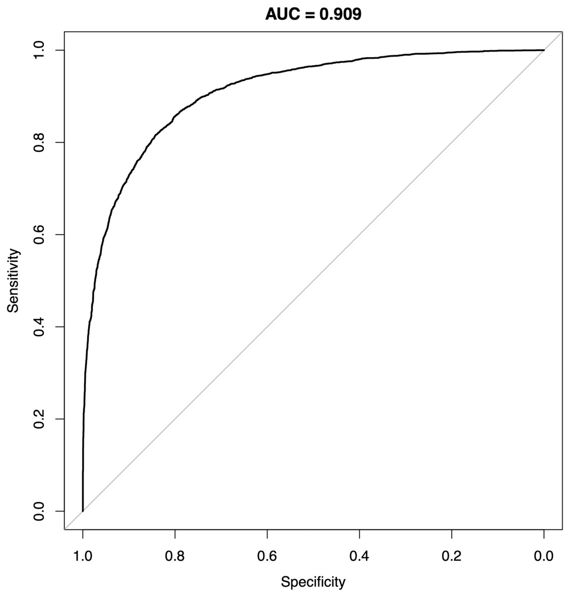
Figure 6: Receiver-operating characteristics of a random forest classifier model for P0 and P1.
Representative result from one SMOTE sampling trial. AUC, area under curve.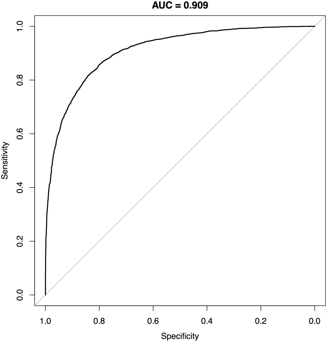
The performance of MB also appeared to improve when oversampling techniques such as SMOTE and machine learning methods such as random forests or neural networks were used; this could potentially aid the algorithmic development for situations where significant imbalance between case and control subjects could occur. For instance, a random forests classifier model trained on the two cohorts using MB element levels alone achieved an AUC of 0.909 (Fig. 6). When compared to a recent report (Kawasaki et al., 2021) comparing the performance of various clinical procedures for colorectal cancer, the AUC of MB outperformed methods such as barium enema (0.836) and even colonoscopy (0.768); in other similarly sized comparisons, MB also appeared to offer above-par performance than other non-invasive tests such as in-stool DNA and fecal immunochemical test (FIT) testing (Imperiale et al., 2014) (0.73 and 0.67, respectively). Especially in “needle in a haystack” situations such as credit card fraud detection or identifying cancer cases in a general population, where incidence rates are typically fractions of a percent, the performance of a model trained with tumor marker panels alone may be highly limited without increasing the dimension of the feature space beyond the typical handful of markers such as CEA, CA19-9 and the like, cohort size constraints will hamper the modeling process. In comparison, MB’s comprehensive ICP-MS profile can be readily expanded at the data reporting stage, thus in a decent-sized cohort fine graining of the feature space may provide improved performance. While next-generation sequencing tools such as whole-exome, whole-genome or even single-molecule real-time (SMRT) sequencing have vastly expanded feature spaces compared to MB, the issue of feature distribution overlap can still exist (Sud, Turnbull & Houlston, 2021), and multigene assays via these sequencing techniques often also involve significantly more human, monetary and infrastructural resources such as multiple sequencers, cloud storage space, technicians and bioinformaticians, etc. (Ignatiadis, Sledge & Jeffrey, 2021) SMRT analysis, for instance, recommends the use of a full computational cluster with upwards of 384 processing cores, 3 terabytes of volatile memory for a single run of sequencing analysis to complete in nearly 7 h (Pacific Biosciences, 2021); at this scale, run time for a study of 8,000 participants by SMRT sequencing-based methods alone will require 6 years of computing time, greatly eclipsing the analytical process of MB.
In addition to the process of establishing case-control discovery studies for the effectiveness of MB screening in a number of different cancer types, we are also contemplating ways to investigate whether MB-like methods can be used for other types of monitoring experiments in specimens such as patient-derived xenografts, or experiments in which connections between particular trace elements with oncogenesis can be confirmed. Aside from bench-scale studies, recently Renatech also independently launched “Metallo-Clinic,” an effort to promote MB screening through Japan. At the time of writing, clinics and testing sites offer MB screening in a number of prefectures covering approximately 52% of the Japanese population (Statistics Bureau of Japan, 2021); if successful, the use and incorporation of MB profiles from Metallo-Clinic may provide a clearer snapshot on true cancer incidence rates in Japan.
Conclusions
In summary, cohort analyses suggested that MB screening was a capable supplementary test to serological tumor marker examinations for a number of cancer types. While the method alone might not be able to discern cancer from non-cancer cases in all situations, depending on the combination of elements, some degree of differentiation still appeared to be possible for cancer type classification. Even in cases where a positive assessment could not be sufficiently determined by the four commonly used tumor markers alone, a number of elements exhibited statistically significant odds between P0 and P1, making the case for referring MB for a secondary confirmation in said situations. Additionally, for both P0 and P1, subpopulations in which tumor markers were within normal ranges, the noticeable distributional differences in elemental levels would again bring emphasis to the implementation of MB in a typical health screening regimen.
As with most epidemiological studies, validation of the collected data remains a difficult hurdle to overcome. While the law of large numbers ensures some degree of reliability and “proximity” of the expected value to the universal truth one seeks, the practical difficulty of having to sift through nominally invariant or average data also increases. Between cohorts P0 and P1, there were significant overlaps in tumor biomarker panel results to make risk assessment based on these markers alone a difficult feat. While cancer biologists and epidemiologists may balk at the idea of utilizing non-conventional observables such as elemental analysis for risk evaluation due to their relative “abstractness” compared to “standards” such as tumor biomarkers or histology reports; nevertheless, it is worthwhile to recognize that those so-called standards may not always be great indicators for all types of cancer. For instance, it has been said that there is lack of sensitivity for CEA during early-stage oncogenesis (Goldstein & Mitchell, 2005), and CA19-9 is not expressed in nearly 5% of the general population (Lamerz, 1999); but as cohort sizes continue to grow, the expandable feature space in novel profiling tools such as MB may finally provide a mean to fill the previously unoccupied void of the early cancer screening feature space.
Supplemental Information
Density Plots of Metallobalance Elemental Level Distribution
File separated by cancer type and gender.
Metallobalance Elemental Analysis and Associated Tumor Biomarker Data
1. Patient ID: newly enumerated without other identifiers (00001, 00002, etc.)2. Cohort ID: P0 (control), P1 (cancer cases) or excluded at subject selection (NA).3. Cancer occurrence: 1 for history of cancer and 0 otherwise.4. Age5. Gender6. ICP-MS levels for the 17 elements tested in metallobalance7. Median tumor biomarker levels.