
Development of a new control rule for managing anthropogenic removals of protected, endangered or threatened species in marine ecosystems
- Published
- Accepted
- Received
- Academic Editor
- Federica Costantini
- Subject Areas
- Conservation Biology, Marine Biology, Mathematical Biology, Environmental Impacts, Population Biology
- Keywords
- Management strategy evaluation, Good environmental status, Cetaceans, By-catch
- Copyright
- © 2024 Ouzoulias et al.
- Licence
- This is an open access article distributed under the terms of the Creative Commons Attribution License, which permits using, remixing, and building upon the work non-commercially, as long as it is properly attributed. For attribution, the original author(s), title, publication source (PeerJ) and either DOI or URL of the article must be cited.
- Cite this article
- 2024. Development of a new control rule for managing anthropogenic removals of protected, endangered or threatened species in marine ecosystems. PeerJ 12:e16688 https://doi.org/10.7717/peerj.16688
Abstract
Human activities in the oceans are increasing and can result in additional mortality on many marine Protected, Endangered or Threatened Species (PETS). It is necessary to implement ambitious measures that aim to restore biodiversity at all nodes of marine food webs and to manage removals resulting from anthropogenic activities. We developed a stochastic surplus production model (SPM) linking abundance and removal processes under the assumption that variations in removals reflect variations in abundance. We then consider several ‘harvest’ control rules, included two candidate ones derived from this SPM (which we called ‘Anthropogenic Removals Threshold’, or ART), to manage removals of PETS. The two candidate rules hinge on the estimation of a stationary removal rate. We compared these candidate rules to other existing control rules (e.g. potential biological removal or a fixed percentage rule) in three scenarios: (i) a base scenario whereby unbiased but noisy data are available, (ii) scenario whereby abundance estimates are overestimated and (iii) scenario whereby abundance estimates are underestimated. The different rules were tested on a simulated set of data with life-history parameters close to a small-sized cetacean species of conservation interest in the North-East Atlantic, the harbour porpoise (Phocoena phocoena), and in a management strategy evaluation framework. The effectiveness of the rules were assessed by looking at performance metrics, such as time to reach the conservation objectives, the removal limits obtained with the rules or temporal autocorrelation in removal limits. Most control rules were robust against biases in data and allowed to reach conservation objectives with removal limits of similar magnitude when averaged over time. However, one of the candidate rule (ART) displayed greater alignment with policy requirements for PETS such as minimizing removals over time.
Introduction
Anthropogenic activities in the oceans are expanding (Halpern et al., 2019; O’Hara, Frazier & Halpern, 2021) and various stressors are responsible for pollution (from contaminants, plastics or noise, among others) and biodiversity loss (Intergovernmental Science-Policy Platform on Biodiversity and Ecosystem Services, 2018; European Commission, Directorate-General for Maritime Affairs and Fisheries, 2023). Ambitious targets and measures are needed to restore biodiversity at all nodes of marine foodwebs (e.g., OSPAR 2021), including apex predators which are often so-called marine megafauna (Authier et al., 2017): these species can integrate changes over large spatial and temporal scales, and can reflect the state of the marine ecosystems. The charisma of sharks, sea turtles, seabirds or marine mammals can capture the attention of citizens and policy-makers to highlight the challenges of biodiversity conservation in the Anthropocene where human activities are largely responsible for their decline (Lewison et al., 2004; Avila, Kaschner & Dormann, 2018; Dias et al., 2019; Pacoureau et al., 2021). Many marine megafauna species are the target of dedicated legislations, be they international, regional or national: these various conservation instruments define them as Protected, Endangered, or Threatened Species (hereafter PETS) depending on their conservation status. In practice, PETS demand measures to ensure their long-term viability in the face of multiple and cumulative pressures (including maritime transport, energy production, tourism, fisheries, aquaculture, and industry).
A major challenge lying at the science-policy interface is defining precisely ‘long-term viability’. Pe’er et al. (2013) numbered some 20 different definitions used in scientific publication to operationalize viability. This profusion can be bewildering to policy makers, managers, or scientists themselves. At its core, viability is a statement about a future state of a population, namely a conjecture that said population will remain in existence over a given period of time, or, equivalently, that it will not go extinct (Ver Hoef, 2006). As such, it is (i) a prediction about an yet-unobserved state of nature, and (ii) it can only be scientifically assessed in the context of a mathematical model that can be unambiguously communicated to decision-makers and specified in a series of unambiguous operations (i.e., an algorithm) to a computer. The latter is necessary to quantify viability, but the former is most critical since an agreement must be reached on what is the desired future state; and it needs to be precisely defined in the form of time-bound conservation objectives (CO).
It cannot be avoided that stakeholders agree on a quantitative formulation of a CO, in order to leverage the effectiveness of mathematics (Wigner, 1960; Hamming, 1980). Mathematical models can be built to encapsulate all current knowledge (including known uncertainties and biases) on a socio-ecosystem to manage (see e.g., European Commission and Directorate-General for Research and Innovation, 2022). Such models are called operating models, or digital twins (Cressie, 2022). An operating model incoporates the best available knowledge and can be put to use for investigating the likely consequences of management actions with numerical simulations. These simulations allow to explore counterfactual scenarios in which different management actions would be carried out, and their consequences are evaluated against a range of performance metrics. This whole approach enables a pro-active approach to conservation: the likely consequences of management actions can be scrutinized ex ante and ranked according to pre-specified requirements in a Management Strategy Evaluation (MSE; de la Mare, 1986; Rademeyer, Plagányi & Butterworth, 2007; Bunnefeld, Hoshino & Milner-Gulland, 2011; Punt et al., 2016; Kaplan et al., 2021). These simulations should not be mistaken for actual measures (which can only be assessed ex post), yet they provide a scientific roadmap for making informed decisions despite considerable uncertainty (Kaplan et al., 2021; Walter III et al., 2023).
For example, Hashimoto, Shirakihara & Shirakihara (2015) investigated the effects of anthropogenic removals, and more precisely by-catch, on the population viability of a marine mammal, the narrow-ridged finless porpoises (Neophocaena asiaeorientalis) in coastal waters around Japan. This cetacean species is Endangered and red-listed by the International Union for the Conservation of Nature (IUCN). By-catch, the unintentional catch of other species during fishing operations targeting commercial species, is a major threat to many marine PETS including cetaceans (Gray & Kennelly, 2018; Brownell et al., 2019). Using population viability analysis (Ver Hoef, 2006) and matrix population models (Caswell, 2006), Hashimoto, Shirakihara & Shirakihara (2015) predicted population size reduction over 30% in half of their numerical simulation trials over the next 100 years. This result was obtained while taking into account uncertainty in the actual magnitude of current by-catch, and illustrates that uncertainty can be factored in and averaged over through numerical simulations.
PETS, by definition, are excluded from direct exploitation, yet they may nevertheless experience additional mortality due to human activities such as by-catch (e.g., small cetaceans, seals, seabirds, turtles, sharks and rays), ship collisions (e.g., baleen whales), collisions with marine renewable infrastructures (e.g., seals, seabirds), habitat destruction and pollution among others. All these activities may lead to anthropogenic removals on marine megafauna populations, that is additional mortality that would not have occurred had human activities not taken place. Conserving marine megafauna and their populations requires to cap these removals and set limits compatible with viability assessments. In the European Union (EU), current legislation requires Member States (MS) to undertake systematic monitoring programme for reliable data collection to estimate the magnitude of removals of, as well as their impacts on PETS populations (European Commission, Directorate-General for Environment, 2021). Despite high ambitions, current mortality monitoring of PETS in the EU (and in North-East Atlantic more broadly) remains largely inadequate to meet these expectations and assess the magnitude of PETS by-catch in fisheries (ICES, 2022; Murphy, Borges & Tasker, 2022; Girard et al., 2022).
Taking stock of both the threats and the lack of legal teeth of several legislations, the European Commission (EC) recently acknowledged “an urgent need to step-up action at EU level to reverse the decline of marine ecosystems by tackling all pressures” (European Commission, Directorate-General for Maritime Affairs and Fisheries, 2023). In particular, the EC calls on EU MS “to develop threshold values for the maximum allowable mortality rate from incidental catches by end of 2023” (European Commission, Directorate-General for Maritime Affairs and Fisheries, 2023). Setting limits to anthropogenic removals of PETS is clearly a salient policy issue (Taylor et al., 2022), as well as one fraught with hurdles. A major one stems from the simple fact that, being non-commercial species, PETS are currently not the primary target of data collection frameworks that can allow routine assessments of the intensity of anthropogenic removals at an ecologically relevant scale. Removals, or even abundance, of PETS are typically known with less precision than those of commercial species whose monitoring is legally required and carried within the Data Collection Framework of the Common Fisheries Policy in EU marine ecosystems for example (https://eur-lex.europa.eu/EN/legal-content/summary/collecting-data-to-assist-in-fisheries-sector-management.html).
In this context of high stakes and low data availability, we carried out in-depth investigations to assess the population viability of PETS in an MSE framework. We focused on cetacean species with which we are most familiar, and for which a large body of work exists. Our results and discussion are, however, not necessarily limited to cetacean or marine mammal species as previous work on marine mammals have been transfered on seabirds or turtles (Dillingham & Fletcher, 2008; Girard et al., 2022). We start by providing a description of relevant international and EU legislations on PETS (including cetaceans) conservation in the North-East Atlantic. We briefly described the MSE framework for assessing the population viability of PETS with a focus on marine mammals and so-called ’harvest’ control rules currently in use. The present paper will not detail operating models for marine mammal population dynamics (Punt, 2016): the interested reader is refered to Genu et al. (2021) for a full description of operating models. We focus on the development of candidate control rules, which we called “Anthropogenic Removals Threshold” (ART), based on a stochastic Surplus Production Model (SPM) that explicitly links removals and abundance of PETS in a simple mathematical model. The use of stochastic SPM models is standard in fisheries management (Polacheck, Hilborn & Punt, 1993; Millar & Meyer, 2000; Bousquet, Duchesne & Rivest, 2008; Bordet & Rivest, 2014). This development section is detailed and primarily intended for mathematical-savvy readers. We finally detailled a desk MSE (sensu Walter III et al. 2023) to benchmark the current and candidate rules with a case study on a small cetacean species in the Northeast Atlantic and discussed of the relevance of simulation testing results with respect to the different control rules available to set removals limits.
Methods
A list of abbreviations and acronyms is provided in Table 1.
| ACRONYM | Meaning |
|---|---|
| ART | Anthropogenic removals threshold |
| ASCOBANS | Agreement on the conservation of small cetaceans of the Baltic, North East Atlantic, Irish and North Seas |
| CO | Conservation objective |
| DCF | Data collection framework |
| EC | European Commission |
| EU | European Union |
| ICES | International Council for the Exploration of the Sea |
| IPL | Internal Protection Level |
| IWC | Internation Whaling Commission |
| MCMC | Markov Chain Monte Carlo |
| MMPA | the United States’ Marine Mammal Protection Act |
| MNPL | Maximum Net Productivity Level |
| MS | Member States |
| MSE | Management Strategy Evaluation |
| OMMEG | OSPAR Marine Mammal Expert Group |
| OSPAR | The (Oslo-Paris) Convention for the Protection of the Marine Environment of the North-East Atlantic |
| PBR | Potential Biological Removal |
| PETS | Protected, Endangered or Threatened Species |
| RLA | Removals Limit Algorithm |
| SPM | Surplus Production Model |
Legislative framework1
The backbone of European legislation on the conservation of wildlife is the Directive on the Conservation of Natural Habitats and of Wild
According to the Marine Strategy Framework Directive (MSFD; Directive 2008/56/EC of the European Parliament and of the Council of 17 June 2008 (https://eur-lex.europa.eu/legal-content/EN/TXT/?uri=CELEX:32008L0056)), priority “should be given to achieving or maintaining good environmental status in the Community’s marine environment, to continuing its protection and preservation, and to preventing subsequent deterioration”. The MSFD requires MS that they monitor the marine ecosystems (Art. 11), including many PETS (as part of the Biodiversity descriptor D1). Reporting is mandatory at the scale of marine sub-regions and, therefore, requires regional coordination. PETS are to be assessed on 5 criteria, including the primary criterion D1C1: “The mortality rate per species from incidental by-catch is below levels which threaten the species, such that its longterm viability is ensured” (https://mcc.jrc.ec.europa.eu/main/index.py). One of the objectives of the Technical Measures Regulation (Regulation 2019/1241; (https://eur-lex.europa.eu/legal-content/EN/TXT/?uri=CELEX:32019R1241)) is to minimise and, where possible, eliminate incidental catches of PETS.
The Oslo-Paris (OSPAR) convention aims at keeping the North-East Atlantic clean, healthy and biologically diverse as well as making it a productive area, used sustainably and resilient to both climate change and acidification (OSPAR, 2021). In particular, OSPAR will work with relevant competent authorities and other stakeholders to minimise and if possible eliminate incidental by-catch of marine mammals, birds, turtles and fish so that it does not represent a threat to the protection and conservation of these species (which are often PETS). The Agreement on the Conservation of Small Cetaceans of the Baltic, North East Atlantic, Irish and North Seas (ASCOBANS) is a conservation agreement under the aegis of the United Nations. The ASCOBANS Conservation and Management Plan, under the heading “Habitat conservation and management” coined the term “unacceptable interaction” (ASCOBANS, 2015). ASCOBANS (2015) defined, according to the best available scientific evidence, “unacceptable interactions” as being, in the short term, a total anthropogenic removal above 1.7% of the best available estimate of abundance (Res.3.3) (https://www.ascobans.org/en/species/threats/bycatch). In practice, this fixed percentage has been used by several EU Member States for setting removals limits on small cetaceans despite well-known shortcomings with respect to the lack of robustness of this method against uncertainty and biases in the data (Winship, 2009). A short description of threshold setting methods can be found in Palialexis et al. (2021), and a more in-depth discussion in the recent OSPAR assessment on cetacean by-catch (Taylor et al., 2022).
The quantitative operationalization of “long-term viability” is enacted in the definition of conservation objectives (a.k.a. conceptual objectives Punt et al., 2016), or so-called ‘policy parameters’. For benchmarking purposes, two conservation objectives will be examined in the remainder, without implying that these choices are prescriptive:
-
the OSPAR Marine Mammal Expert Group (OMMEG)’s interpretation of the ASCOBANS conservation objective to restore or maintain population size to at least 80% of carrying capacity (hereafter denoted K) over a time horizon of 100 years with the probability of 0.8 (COOMMEG; Genu et al., 2021; Taylor et al., 2022);
-
to restore or maintain population size to at least 60% of carrying capacity (K; see below) over a time horizon of 50 years with the probability of 0.9 (COtMNPL).
COOMMEG enabled to carry out an assessment of anthropogenic removals of marine mammals in the North-East Atlantic (Taylor et al., 2022); but has also been challenged on several grounds (M Authier, pers. obs., 2021-2022) including
-
a lack of ambition because the time horizon is too distant;
-
too much ambition because 80% of K is too conservative;
-
a lack of precaution because a risk of failing the conservation objective of 0.2 is too high;
-
too much precaution because a probability of 0.8 is too high.
To partly address these challenges and knowledge gaps, we investigated also COtMNPL where tMNPL stands for ‘theoretical Maximum Net Productivity Level’, defined as a population experiencing density-dependence being above its Maximum Net Productivity Level (MNPL), which is thought to be 60% of carrying capacity for marine mammals (Taylor & Demaster, 1993; Zerbini et al., 2011; Guilherme et al., 2021). COtMNPL lowers the target, time horizon and risk compared to COOMMEG. CO are best viewed as ‘policy parameters’ emerging from a consensus on the appropriate level of ambition sought by parties and informed by current scientific evidence and knowledge.
Notations
Notations are summarized in Table 2. Let denotes the log-normal distribution of parameters location and scale. Let denotes the uniform distribution bounded by parameters lower and upper. The notation flags an estimate of a parameter, which can be the a posteriori mean or some quantile from a posterior distribution.
| Name | Type | Meaning |
|---|---|---|
| K | Integer | Carrying capacity (same unit as Nt, or Rt) |
| Nt | Integer | True abundance (in number of individuals) at time t |
| Integer | Observed abundance (in number of individuals) at time t | |
| cvt | Positive real | Coefficient of variation associated with |
| Rt | Integer | Removals (in number of individuals) at time t |
| Dt | Positive real | Depletion at time t: ratio of Nt over K |
| ρt | Positive real | Removal rate at time t |
| r∗ | Positive real | Population growth rate at the MNPL |
| r | Positive real | Current population growth rate |
| MNP | Positive real | Maximum Net Productivity: |
| the maximum possible per capita rate of increase per year | ||
| MNPL | Proportion | Maximum Net Productivity Level |
| z | Positive real | Shape parameter of the Generalized Logistic Population Growth model |
| rmax | Positive real | Maximum theoretical or estimated productivity rate; related to MNP |
| FR | Proportion | Recovery factor |
| Nmin | Integer | Minimum population estimate |
| IPL | Proportion | Internal Protection Level; a fraction of K |
| wt | Positive real | weight for the likelihood (Eq. 9) |
| cvσ | Positive real | Coefficient of variation associated with environmental stochasticity |
| ɛt, σ | Positive real | Environmental stochasticity |
Management strategy evaluation
Management procedures for cetaceans have been developed, in particular within the work of the IWC (Punt et al., 2016; Punt, 2019). A management strategy is a set of rules which aim at making agreed-upon objectives achievable (Punt, 2006; Rademeyer, Plagányi & Butterworth, 2007; Bunnefeld, Hoshino & Milner-Gulland, 2011; Punt et al., 2016). This strategy defines management objectives in the form of not-to-be exceeded thresholds that managers can track from available data. The process of evaluating a management strategy (MSE) relies on modeling and computer simulations (de la Mare, 1986; Cooke, 1994; Hilborn & Mangel, 1997; Rademeyer, Plagányi & Butterworth, 2007; Punt et al., 2016). In order to carry out these simulations, MSE heavily leans on models, especially on so-called operating model.
MSE is commonly used to compute biological reference points or, in the context of PETS, removals limits. Removals limits are determined for the use of so-called ’harvest’ control rule which is a mathematical formula or model taking available data as inputs. Below we described two commonly used control rules for managing marine mammals. However, a complication in the management of PETS stems from the fact that PETS removals, unlike commercial species’ catch, are not usually monitored (no logbooks). For example, data on PETS by-catch is not systematically collected by onboard observers: these data, if not collected systematically and in a dedicated scheme, are usually of low quality and biased (Basran & Sigursson, 2021). This is especially true in European waters where there are no dedicated schemes to monitor by-catch at the relevant scales, especially marine mammal by-catch (Murphy, Borges & Tasker, 2022).
Operating models
An operating model is a “digital twin” of the socio-ecosystem to be managed. It is a mathematical (and hence idealized) representation of the phenomenon under study that encapsulates important knowledge about the phenomenon (Punt et al., 2016), in this case population dynamics of PETS. In the case of cetaceans, commonly used operating models include a population dynamics model that can be age-aggregated (Wade, 1998; Wade, 2002) or age-disaggregated (Wade, 2002; Brandon et al., 2017). The interested reader is referred to Punt (2016) for a review of operating models developed for cetaceans; to Tuck (2011) and Tinker et al. (2022) for seabird operating models; and to Chaloupka & Balazs (2007) and Snover (2008) for a discussion on a turtle operating model. These operating models are variants of SPM. In the remainder, the operating model is age-disaggregated (that is age-structured), it assumes a Pella-Tomlinson functional form for density-dependent fecundity (see Algorithm 2 in Genu et al., 2021 for a full description of the model) and no Allee effect (see e.g. Haider et al., 2017).
Control rules for managing removals
There are two main control rules currently used for managing marine mammal removals: the Potential Biological Removal (PBR; Wade, 1998) and the Removals Limit Algorithm (Cooke, 1995).
Potential Biological Removal
The calculation of the PBR is straightforward (Wade, 1998): Nmin being an estimate of minimum population size, one half of the maximum theoretical productivity rate of the stock and FR a recovery factor chosen between 0.1 and 1. The computation of PBR does not require data on removals, although they are necessary to gauge the level of removals against the PBR limit (that is, to carry out an assessment). PBR is extensively used in the United States where it is enshrined in the US Marine Mammal Protection Act (MMPA). It has also been used in several cases, including dolphins, for example in New Zealand (Slooten & Dawson, 2008) or in the EU (e.g., Baltic harbour porpoise Berggren et al., 2002; grey seal Halichoerus grypus Taylor et al., 2022; common dolphin Delphinus delphis ICES, 2020).
Removals limit algorithm
The other harvest control rule currently in use is known as the Removals Limit Algorithm (RLA; Winship, 2009; Hammond, Paradinas & Smout, 2019). It also aims at setting an upper limit to anthropogenic mortality of PETS, and was applied to the population of Harbour porpoise in the North Sea (Hammond, Paradinas & Smout, 2019; Genu et al., 2021; Taylor et al., 2022). The RLA requires both a time-series of abundance/biomass estimates (whereas PBR only requires one such estimate) and a time-series of removals (whereas PBR requires none for its computation). RLA is a variant of the Catch Limit Algorithm (CLA), formulated by Cooke (1994) for baleen whales (Internation Whaling Commission, 2012). The RLA is an ad hoc algorithm that uses historical series of captures and estimates of abundance (Hammond, Paradinas & Smout, 2019): (1)
where Nt and Rt are respectively the abundance/biomass and removals at time t. The computation of the RLA control rule for setting a removals limit (as a fraction of the best available abundance estimate) is: (2)
where T stands for the current year, DT is the current depletion (that is, , K being the carrying capacity) and IPL (Internal Protection Level) is the depletion threshold below which the limit is set to 0 (Punt, 1993). Both r and DT are estimated from the model defined by Eq. (1) in a Bayesian framework (Hammond, Paradinas & Smout, 2019; Genu et al., 2021) and removals limit is computed from the joint posterior distribution of (r, DT). A point estimate is used in practice by selecting a quantile of the posterior distribution of the removal limit to account for uncertainty.
Candidate control rules
The PBR control rule takes a value for rmax as an input while the RLA control rule uses a posterior distribution of r (from Model 1). For most species, rmax or r are unknown in practice, and a default value can be used for PBR, or r needs to be estimated from a prior and data. This knowledge gap (unknown rmax or the choice of the prior for r) may be exploited to argue against the use of either of these rules using uncertainty distortion strategies (Schweder, 2000; Rayner, 2012). Devising a new rule to set a removals limit that does not directly hinge on knowledge of this input is thus desirable to (i) avoid any strategic mis-representation of uncertainty during the policy process (see more generally Rayner 2012); and (ii) diversify options for discussions during the policy process. We developed candidate control rules based on the same data requirements as the RLA, namely a time-series of removals and at least one estimate of abundance that are fed into a statistical model (Hammond, Paradinas & Smout, 2019; Genu et al., 2021). The statistical model is however different in how it incorporates the removals data. In Eq. (1), removals are treated as a known covariate. Below, we developed a stochastic model for removals directly.
Development of a stochastic SPM
Population models for PETS are often based on SPM (e.g., Snover, 2008; Punt, 2016) which are standard models of population dynamics in situations of strong uncertainty and low information. SPMs seek to encompass important population processes governing the dynamics of abundance change over time (Hilborn & Walters, 1992; Ver Hoef, 2006):
In particular, density-dependence in paramount to take into account (Punt, 2016): a convenient functional form is that described by Pella & Tomlinson (1969), assuming a first-order Markovian process on abundance: (3)
Setting z = 1 gives the well-known Schaefer model in fisheries (Schaefer, 1991), and Nt and Rt are respectively the abundance/biomass and removals at time t, K being the carrying capacity and r∗ the growth rate at the Maximum Net Productivity Level (MNPL; r∗ is also known as the Maximum Sustainable Yield Rate).
Incorporating environmental variability (the so-called process noise ɛt) in a multiplicative way in Eq. (3) yields (Polacheck, Hilborn & Punt, 1993; Millar & Meyer, 2000): (4) This shift to a stochastic framework, assumed to be more realistic for describing changes in abundance, implies that the {Nt} states are random variables, similar to ɛt. At time t, the noise ɛt is classically assumed to be unbiased and homoskedastic (and therefore independent on t and past random variables (removals, abundances, noises):
Assuming a simple relationship between removals Rt and abundance Nt: (5) where is a time-invariant removal rate (Bousquet, Duchesne & Rivest, 2008; Bordet & Rivest, 2014), the removal process becomes: (6)
The set of parameters in Eq. (6) is defined as . Parameter z is usually fixed rather than estimated (Fletcher, 1978; Best & Punt, 2020). For example, setting z = 2.39 corresponds to a MNPL of 60% of K that is customarily assumed for marine mammals (Punt, 2016; Kanaji et al., 2021).
Equation (5) is a simplifying assumption that allows to link the abundance and removal processes. Stochasticity is introduced in Eq. (6) which allows to write a likelihood function (see below and Supplementary Information Appendix 1) for estimating a removal rate from data. In particular, it allows a time-series of past removals to be analyzed as the response variable where most current approaches treat these removal data as covariates (e.g., Kanaji et al., 2021). In effect, this choice means that removals are used as an index of abundance.
Reparametrization
Following the reparametrization of Bordet & Rivest (2014), let which is well defined for z − ρz + r∗(1 + z) > 0, that is With z > 0 this assumption is not restrictive since 0 < ρ < 1. Eqs. (4) and (6) can be re-arranged: with Zt = D(θ)Rt and Note that positive removals imply . To simplify notations and to adopt a more conventional Markovian writing, we rewrite: (7) where (8) Note that g is neither linear nor log-linear. Appendix 1 in the Supplementary Information details the likelihoods for estimating θ from data. In the remainder, we denote ℓ({Rt}|θ) the likelihood associated with removals.
Initial conditions
For practical reasons, the initial depletion D0 at the start of the time-series of removals, instead of K, is estimated. This choice is convenient as . Initial abundance N0 is typically unknown for PETS and the first abundance estimate available may not even match the start of the observed removals time-series. In that case, information on initial depletion D0 may be elicited from expert knowledge (see e.g., Bockting, Radev & Brükner 2023) or historical data, and given a prior distribution: it may be easier to elicit a prior on depletion (a quantity expected to be bounded between 0 and 1) than on K directly. In practice, K is deduced from D0 and the first observed abundance estimate that is available (e.g., Punt, 2019). The set of parameters to estimate is now: θ = {r∗, σ, ρ, D0}. The stochastic SPM defined above (Eqs. 6 & 8) was implemented in the probabilistic programming language Stan (see Appendix 2; Carpenter et al., 2017).
Anthropogenic removals threshold (ART)
The stochastic SPM developed above meshes removal and abundance processes by assuming a crude proportionality between the two, which is simplistic but aligns with stakeholder perceptions of variations in PETS by-catch for example (M Authier, pers. obs.). It is not a realistic model as removals depends strongly on fishing effort, which in turn is influenced by a myriad of factors. However, as Rademeyer, Plagányi & Butterworth (2007) noted, “[e]stimators based on simple population models have often been shown to perform as well or better than those based on more complex ones”. We are thus less interested in biological realism than in the performance of this model for management.3 The stochastic SPM assumes stationarity (that is time-invariance) in ρ, the removal rate, which is at odds with the very purpose of managing removals. If management is meant to be effective, it will take action to precisely change the level of removals. By definition, management aims at changing ρ over time so the model is clearly wrong once management is implemented. Before management is implemented, stationarity is an assumption as there is typically little knowledge or data are too noisy to test it. To obviate this issue while retaining a parsinomious model with four parameters, we used a statistical estimation paradigm based on the notion of weighted (or local) likelihood (Tibshirani & Hastie, 1987; Wang, 2006; Agostinelli & Greco, 2013). This approach allows us to progressively down-weigh data extending the furthest back in time (i.e., to consider that the policy relevance of statistical information provided by each datum in a sample depends on how far back in time the datum was collected). Applied only to the likelihood of removals, it is formalized as follows (see Appendix 1): the likelihood ℓ({Rt}|θ) is replaced by
(9)
where the weights wt(η) have the sense of kernels, i.e., they provide a kernel-based representation of the score function In choosing the weights wt(η), such that the above representation has good convergence properties, the following properties must hold (Agostinelli & Greco, 2013): wt(.) should be a bounded differentiable non-negative function of t that may depend on a parameter η which can be consistently estimated by , such that where c is a positive constant. The following choice (Gaussian kernel): obeys these requirements (with c = 1), provided the scale parameter η be estimated by some rule that favors the information provided by the sample of most recent observations in the estimation of θ, trading bias for precision (Hu & Zidek, 2002).
In this study, η was chosen so that data older than 50 years contribute less than 0.05 to the likelihood during estimation (wt = 0.05 for (t − 50)). This choice (η = 20.4) is arbitrary but was found to work well in practice (see Results). In addition, a sample size of 50 appears adequate for our purposes (although smaller sample size could work but this point requires additional simulations).
Capitalizing from the stochastic SPM (Eq. 9), we propose two candidate control rules (as a fraction of the best available abundance estimate) which we call Anthropogenic Removals Threshold (ART) to emphasize that the quantity derived from these control rules represents a threshold beyond which conservation objectives run a high risk of not being met.
The first candidate is simply the posterior mean of the quantity: (10)
where FR is a recovery factor chosen between 0.1 and 1 (as in the PBR control rule). This rule adapts the historical removal rate and does not directly rely on an estimate of carrying capacity or population growth rate as the RLA control rule (although both a carrying capacity and a population growth rate are in θ). The second candidate is an elaboration that takes into account any trend in abundance, and more specifically any evidence of a decline, to negatively feedback on the removals limit: (11)
where β is a trend in abundance (on a logarithmic scale) estimated using the regularized approach detailed in Authier et al. (2020). Briefly, β is the slope of a regression line through the abundance estimates (scaled by the first estimate and then log-transformed) and estimated using a weakly-informative prior (namely the ‘skeptical’ prior of Cook, Fúquene & Pericchi, 2011) that favours the hypothesis of no trend over time (see Authier et al., 2020 for an in-depth investigation of this choice in the context of trend estimation). This candidate rule operationalizes the principle on non-deterioration whereby populations or species in need of restoration (that is, that are depleted) should not be allowed to deteriorate further. If no trend or a positive trend in abundance is evidenced, candidate2 is equivalent to candidate1. Both candidate1 and candidate2 can be computed for the same data necessary to compute RLA, and their posterior mean approximated by the average over MCMC samples of the posterior distribution after estimating θ from data (see Appendices 2 and 3).
Simulations
The operating model used in population dynamics simulations was a stochastic and age-disaggregated version of a generalized logistic model of population dynamics (Punt, 2016) as implemented on the R package RLA v.0.2.0 (Genu et al., 2021). Given initial conditions, biological parameters and removals, abundance data are generated at each time step. The model aims to mimic the population dynamics of a small-sized cetacean (Fig. 1).
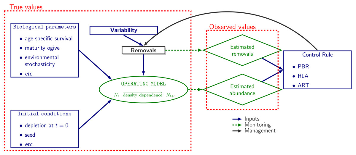
Figure 1: Simulation workflow.
Schematic representation of the workflow for simulations. Population dynamics (N denotes abundance) are simulated from biological parameters (life-history data, true removal rate etc.). Monitoring allows to collect data but these data are noisy: they always include observation noise and, depending on robustness trials, can be biased (see Genu et al. 2021 and R code provided in the supplementary materials). Data are used as inputs in control rules for managing removals.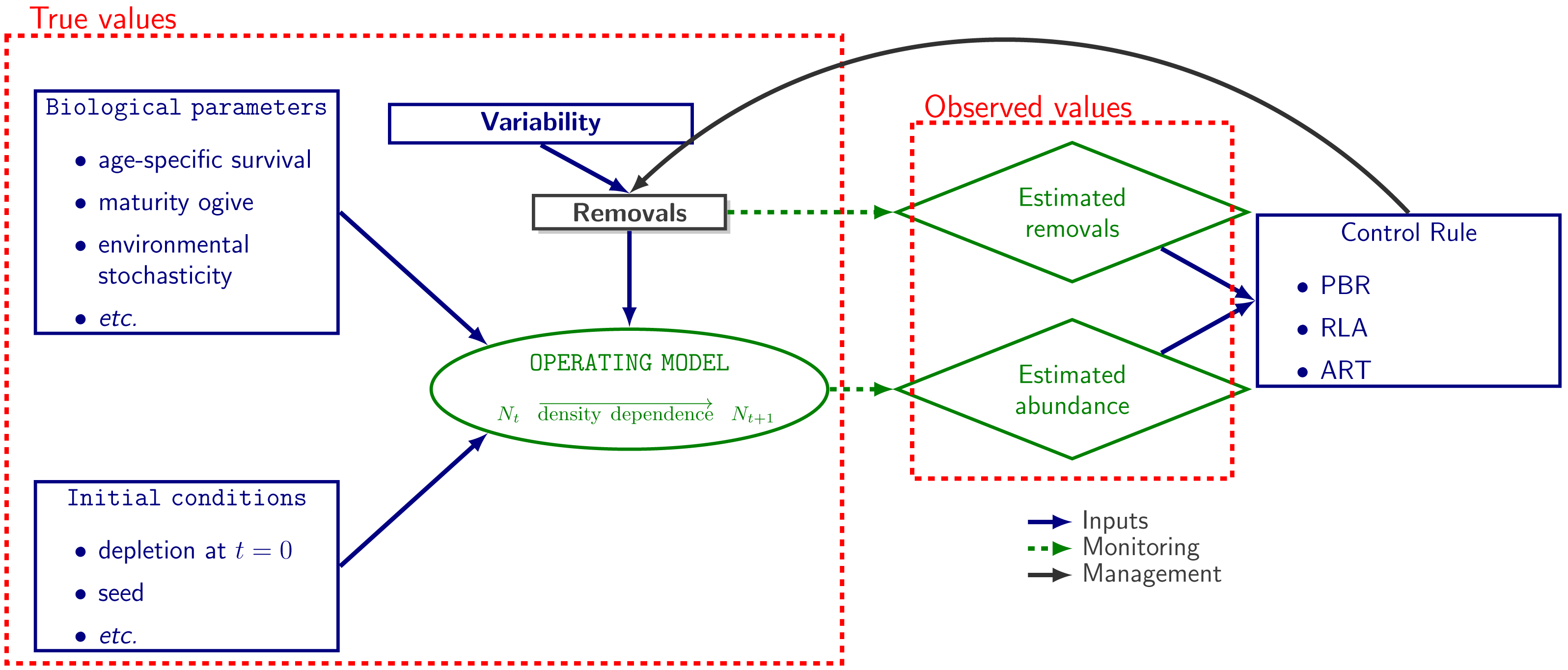
Life-history parameters were set to those of a small-sized cetacean species, the harbour porpoise (Phocoena phocoena) in the North Sea (Hammond, Paradinas & Smout, 2019). A hundred (100) simulations were carried out: for each a hypothetical population of harbour porpoises was depleted with unmanaged anthropogenic removals for 50 years before implementing management procedures and specific control rules (see below). A time-series of removals as long as 50 years is unusual in general, but one is available for harbour porpoise in the North Sea (Hammond, Paradinas & Smout, 2019). For benchmarking purposes with previous similar MSE (Hammond, Paradinas & Smout, 2019; Genu et al., 2021), we kept this assumption of a depth of 50 years for the removals time-series at the beginning of management.
A distribution of initial depletion levels was induced between 30% and 60% (Fig. 2). Important biological inputs include the Maximum Net Productivity (MNP) and MNPL, which are usually unknown in most cases. To reflect that uncertainty, a range of plausible values for small cetaceans (Taylor & Demaster, 1993; Wade, 1998) were considered (Fig. 2).
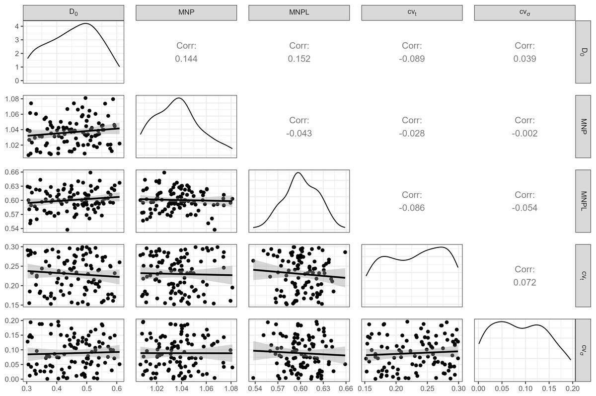
Figure 2: Inputs for the operating model.
100 weakly-correlated values for Maximum Net Productivity (MNP), Maximum Net Productivity Level (MNPL), initial depletion, observation error (cvt) and environmental stochasticity (cvσ) were drawn at random and used for MSE. Pearson correlation coefficients are displayed above the diagonal.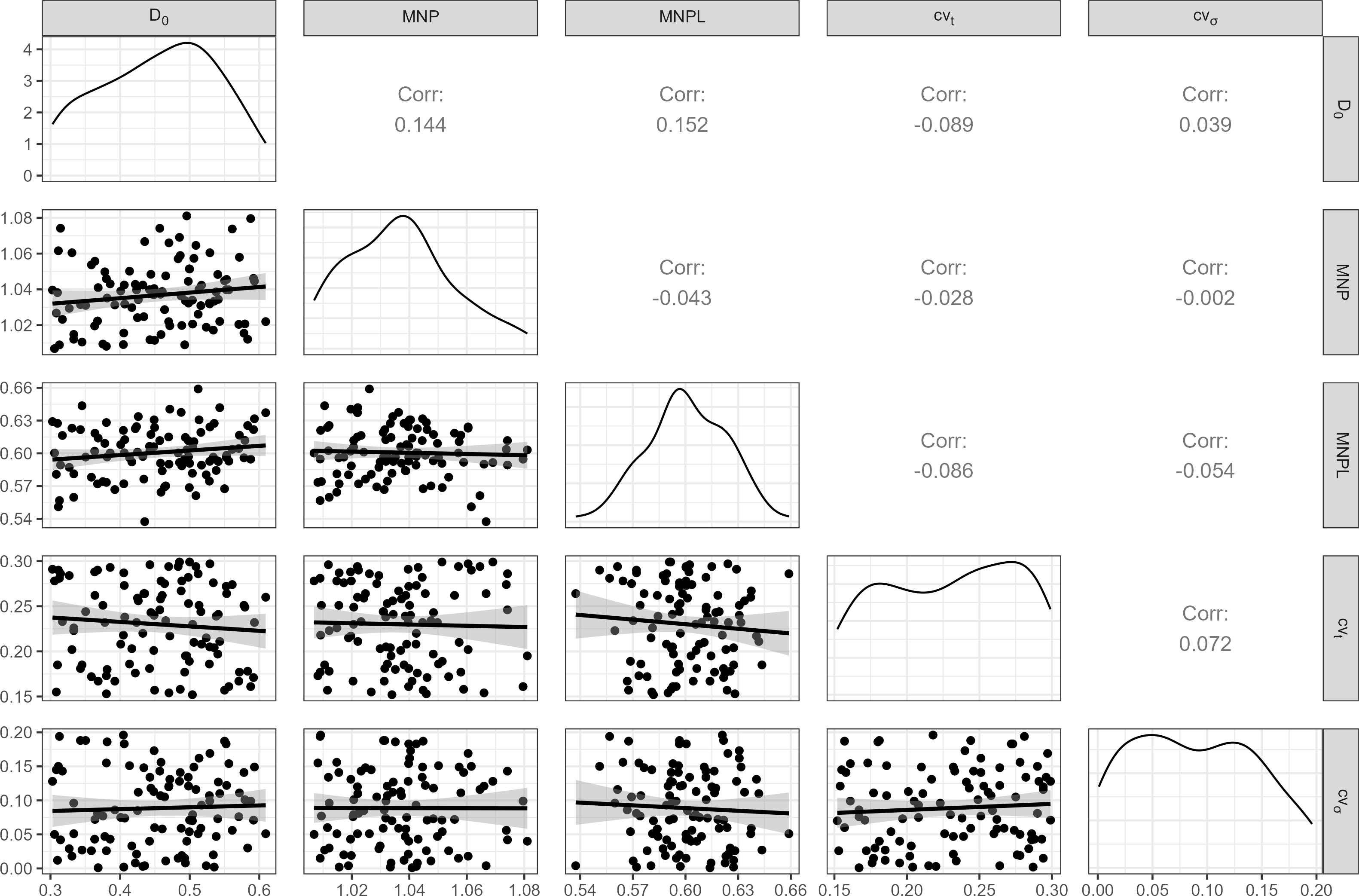
(‘Harvest’) control rules
We tested five control rules for managing anthropogenic removals of PETS:
-
the fixed percentage rule of ASCOBANS (2000): ;
-
the PBR rule of Wade (1998) with Nmin defined as the 20% quantile of a log-normally distributed abundance estimate : ;
-
the RLA rule, with ;
-
the candidate1 ART, with ; and
-
the candidate2 ART, with .
To set a removals limit, the fixed percentage rule of ASCOBANS (2000) only requires a point estimate of current abundance requires a recent point estimate of abundance and its associated coefficient of variation to compute an estimate of minimum population size Nmin. The rules RLA and ARTi∈[1:2] each require a time-series of abundance estimates with their uncertainties as well as a time-series of removals’ estimates. All rules, save for the fixed percentage one (which was included as a negative control), need tuning. For PBR, ART1 and ART2, this process means the testing of different values of FR to identify the minimum one that allows to reach a given CO. For RLA, tuning is achieved by testing different quantiles of the posterior distribution of Eq. (2) (Genu et al., 2021). That quantile tuning was not carried out with ART1 or ART2 stemmed from the typically tight posterior concentration observed when estimating ρ during the development of the stochastic SPM (Ouzoulias, 2022). In contrast, posterior concentration does not occur because the log-normal likelihood assumed for Eq. (1) when estimating removals limit is down-weighted by a fixed factor to limit the speed at which the management procedure responds to feedback (Cooke, 1999).
Scenarios
We evaluated control rules on three scenarios: a base case scenario whereby unbiased but noisy data are assumed to be available and collected; and two so-called robustness trials. In the first robustness trial, estimates of abundance were assumed to be observed with a systematic bias resulting in an overestimation by a factor 2. In the second, removals’ estimates were assumed to be biased downward, resulting in an underestimation of true removals by a factor 2. The two robustness trials were found to be the most challenging ones in a previous investigation (Genu et al., 2021).
Performance metrics
The effectiveness of control rules to meet requirements of management was gauged on 6 performance metrics. A period of 6 years was chosen to match the reporting cycle for the MSFD. Accordingly, it was assumed during simulations that abundance estimates would be updated every 6 years. The first performance metric allows tuning by selecting either a value for FR or a quantile for each control rule in order to meet a CO. The second allowed a comparison with the fixed percentage rule of ASCOBANS. The third and fourth metrics informed on the variability in removals limits for a given control rule, with greater stability with low cv and positive autocorrelation. The fifth indicated any systematic changes in removals limits over time: it is the estimated slope of a linear regression of the computed removals limit against time with time rescaled to the unit interval (the model was fitted using the default settings of function stats::lm in R version 4.2.2) (R Core Team, 2022). This performance metrics reveal how the removals limit is changing on average over time (increasing, decreasing, no change) as it is updated every 6 years in light of monitoring data. The sixth performance metric informed on the expected delay in population recovery, where recovery was defined as the time at which a CO was sustained over 6 consecutive years (to match the MSFD reporting cycle). The performance metrics were:
-
the level of population (true) depletion at the end of each simulation;
-
the average removals limit (average, as a percent of current abundance estimate) across simulations;
-
the coefficient of variation (cv) of removals limits computed within each simulation and averaged over simulations;
-
the 1-lagged autocorrelation (autocorrelation) in removals limits computed within each simulation and averaged over simulations;
-
the temporal trend (trend, in %) in removals limits within a simulation and averaged over simulations; and
-
the average delay in recovery (delay, in years) compared to a hypothetical complete ban on removals.
Implementation
To carry out a (desk) MSE, we used a cross-factorial design with two CO, five control rules, three scenarios, 10 FR and 100 simulations. The total computational budget was 30, 000 runs which were sent to the computing cluster Curta hosted at Bordeaux University, France. Computer time for this study was provided by the computing facilities of the MCIA (“Mésocentre de Calcul Intensif Aquitain”). All simulations were carried out using the functionalities of the dedicated R package RLA v.0.2.0 (Genu et al., 2021) available at https://gitlab.univ-lr.fr/pelaverse/RLA. The different functions used are mentioned in Table 3. As simulations rely on random numbers, seeds were controlled for and recycled across control rules within scenarios in order to match and compare results (Rademeyer, Plagányi & Butterworth, 2007).
| Control rule | Data | Model | Function | Stan |
|---|---|---|---|---|
| requirements | dimensionality | name | model code | |
| Fixed percentage | at least one | 0̸ | fixed_percentage | 0̸ |
| PBR | abundance estimate | pbr_nouveau | ||
| RLA | time-series of | 2 | forward_rla | uniform |
| ART1 | both removals and | 4 | art_nouveau | sspm |
| ART2 | abundance estimates | 6 | sspm_trend |
Computation of PBR does not require any model fitting in contrast to RLA and all flavours of ART which have an estimation step for quantities of interest to compute removals limits. With a time horizon of 100 years and an assumed frequency of 6 years (as per MSFD cycle), model fittings are required within one run. Estimation of θ (Appendices 2 and 4) was carried out in a Bayesian framework using programming language Stan (Carpenter et al., 2017) called from R v.4.2.2 (R Core Team, 2022) with library Rstan (Stan Development Team, 2023). Four chains were initialized and run for a total of 2,000 iterations, discarding the first 1,000 as warm-up and retaining every 1 iterations (no thinning). Control parameters for the No-U-Turns algorithm were kept to their default values. Parameter convergence was assessed using the statistics (Vehtari et al., 2019) and assumed if .
Results
The ASCOBANS rule of 1.7% of best available abundance estimate (a total anthropogenic removal above 1.7% of the best available estimate of abundance) allowed depleted populations to recover to either 60% or 80% of K with a probability above 0.5 in the base scenario only (Table 4; Appendix 3). These probabilities did not rise to the nominal levels set by either of the COs in any of the scenarios: this rule failed to meet CO and was not robust against biases in either the abundance or removal data. For the medium to small number of simulations in which COs were reached, the average delay in recovery was between 5 and 25 years compared to a hypothetical complete ban on removals.
| Conservation objective | Scenario | Recovery rate | Delay (years) |
|---|---|---|---|
| COOMMEG | Base case | 0.60 | 14.1 |
| Overestimated abundance | 0.19 | 24.6 | |
| Underestimated removals | 0.19 | 24.6 | |
| COtMNPL | Base case | 0.71 | 4.6 |
| Overestimated abundance | 0.38 | 9.1 | |
| Underestimated removals | 0.38 | 9.1 |
The fixed percentage rule has no free parameter to tune, in contrast to other rules (Fig. 3). Tuning these rules to COs is summarized on Fig. 3. As expected, lower tuning values were selected in robustness trials compared to the base case scenario with no biased data. An evaluation of the ART1 control rule could not be completed for the scenario in which abundance was systematically over-estimated as simulations stopped due to numerical issues in model fitting. As a result, this control rule was not robust against overestimated abundance as it could not be used in this scenario. The difference in tuning parameters for PBR, RLA and ART was modest between COs (compare Figs. 3A and 3B). In contrast, the value for FR was halved when swapping COOMMEG for COtMNPL (compare Figs. 3A and 3B).
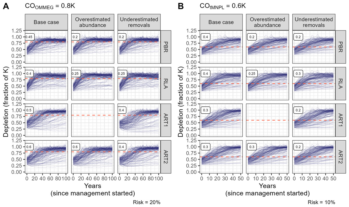
Figure 3: Tuning the control rules.
(A) Tuning with respect to the OMMEG interpretation of the ASCOBANS CO: to restore population to 80% of K with probability 0.8 in 100 years. (B) Tuning with respect to a CO of restoring population to a theoretical MNPL of 60% of K with probability 0.9 in 50 years. Labels in the upper left corner of each sub-panels correspond to tuning and display the largest value of Fr (PBR, ART1, ART2) or the largest quantile (RLA) that achived a given CO.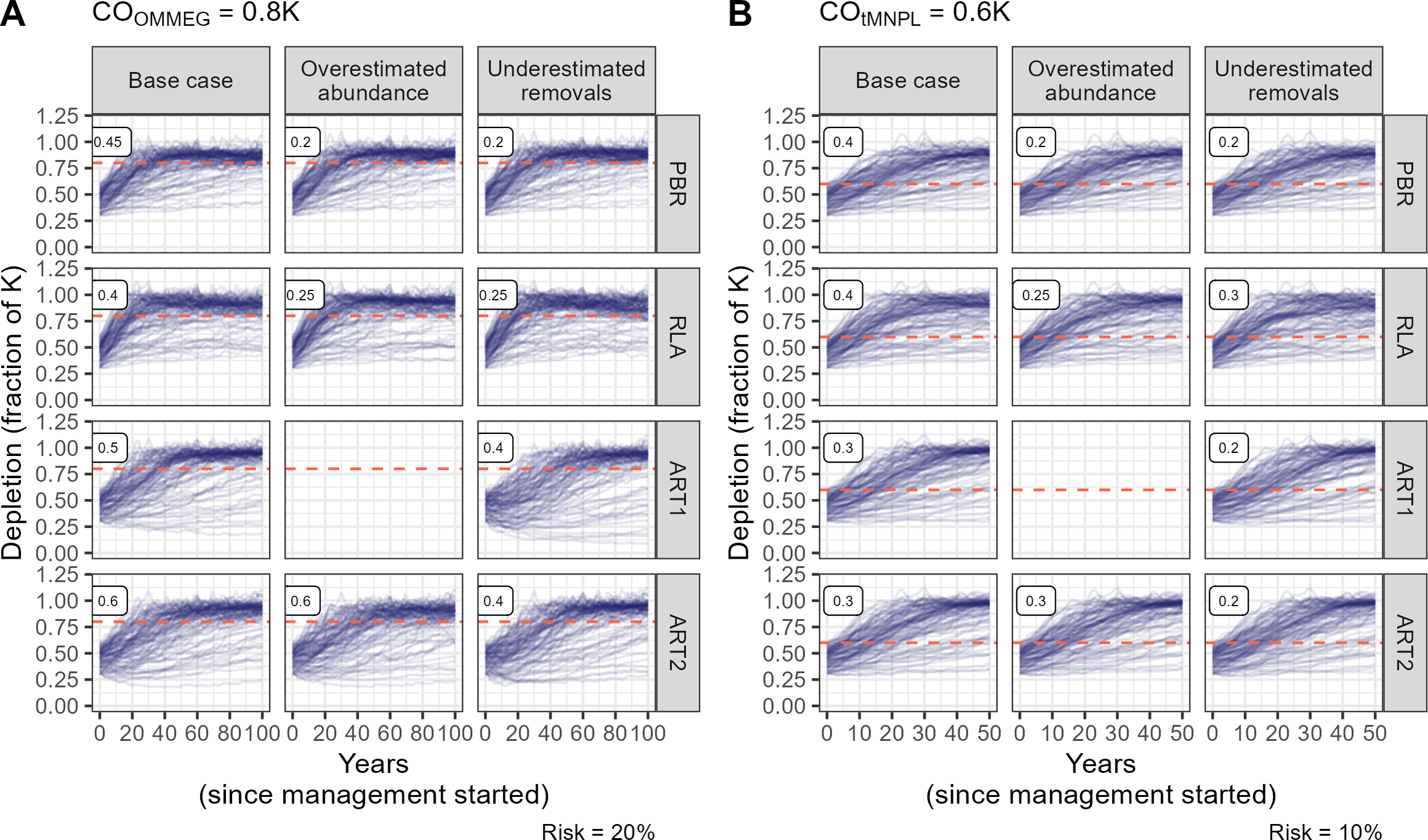
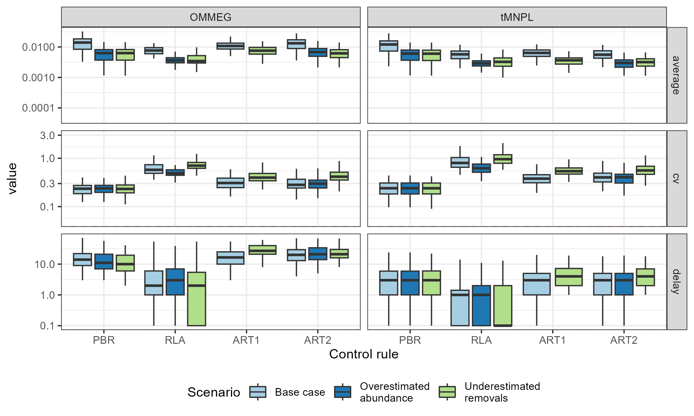
Looking at performance metrics (Table 5 and Fig. 4) (see also Appendix 4), average removals limits were similar across the different control rules: they were, on average, never larger than the ASCOBANS fixed percentage of 1.7%, and smaller than 1% in general. The greatest variability (cv) in these limits was associated with RLA, and the smallest with PBR, with ART in-between. The scenario in which removals were underestimated displayed the largest volatility in removals limits, a result that held across the different rules. Delays in recovery, relative to a complete banning of removals, were the longest with the use of ART1 or ART2, and the shortest with the use of RLA.
| Conservation objective | Control rule | Scenario | Performance metrics | ||||
|---|---|---|---|---|---|---|---|
| cv | Autocorrelation | Average | Delay | Trend | |||
| COOMMEG | PBR | Base case | 0.24 | −0.13 | 0.014 | 16.5 | 3.6 |
| Overestimated abundance | 0.24 | −0.10 | 0.006 | 14.3 | 3.7 | ||
| Underestimated removals | 0.24 | −0.07 | 0.006 | 12.9 | 3.6 | ||
| RLA | Base case | 0.65 | 0.34 | 0.008 | 5.1 | 8.1 | |
| Overestimated abundance | 0.51 | 0.28 | 0.004 | 4.8 | 6.6 | ||
| Underestimated removals | 0.79 | 0.37 | 0.004 | 3.3 | 9.7 | ||
| ART1 | Base case | 0.32 | 0.70 | 0.011 | 18.7 | −4.2 | |
| Underestimated removals | 0.44 | 0.69 | 0.008 | 29.4 | −5.9 | ||
| ART2 | Base case | 0.36 | 0.68 | 0.013 | 23.4 | −3.3 | |
| Overestimated abundance | 0.35 | 0.63 | 0.007 | 25.0 | −1.7 | ||
| Underestimated removals | 0.48 | 0.65 | 0.007 | 23.8 | −5.5 | ||
| COtMNPL | PBR | Base case | 0.24 | −0.11 | 0.012 | 3.8 | 3.7 |
| Overestimated abundance | 0.24 | −0.11 | 0.006 | 3.8 | 3.7 | ||
| Underestimated removals | 0.24 | −0.15 | 0.006 | 3.7 | 3.6 | ||
| RLA | Base case | 0.90 | 0.31 | 0.006 | 0.2 | 8.1 | |
| Overestimated abundance | 0.65 | 0.32 | 0.003 | 0.3 | 6.6 | ||
| Underestimated removals | 1.05 | 0.25 | 0.003 | 0.3 | 8.8 | ||
| ART1 | Base case | 0.39 | 0.54 | 0.007 | 3.7 | −6.4 | |
| Underestimated removals | 0.56 | 0.51 | 0.004 | 4.7 | −5.2 | ||
| ART2 | Base case | 0.43 | 0.53 | 0.006 | 3.1 | −5.7 | |
| Overestimated abundance | 0.43 | 0.53 | 0.003 | 3.4 | 0.6 | ||
| Underestimated removals | 0.59 | 0.50 | 0.003 | 4.1 | −4.2 | ||
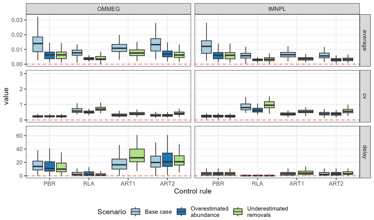
Figure 4: Performance metrics.
Boxplots summarizing the distribution of variability (cv, unitless), mean (average, as a proportion of current abundance estimate; e.g., 0.01 = 1%), and delay in recovery (in years). See Appendix 4 for the same plot with a logarithmic scale on the y-axis.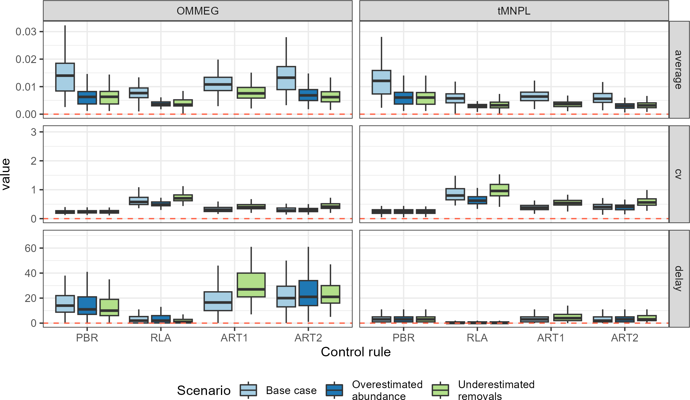
With respect to autocorrelation, there was a clear gradient across control rules, with an increase from PBR to ART2 (Table 5 and Fig. 5). The largest positive autocorrelation was evidenced from setting limits with the stochastic SPM: two successive limits were more similar to each other when set with ART1 or ART2 compared to one set by either RLA or PBR. In that latter case, autocorrelation was nil or tended to be negative. With respect to trend in removals limit within a simulation, it was positive when using either RLA or PBR: removals limits tended to increase over time. In contrast, the trend was negative when using either ART1 or ART2: limits decreased on average over time in these cases. Results from a single simulation (using the same seed for random number generation) is depicted on Fig. 6 (see also Appendix 5).
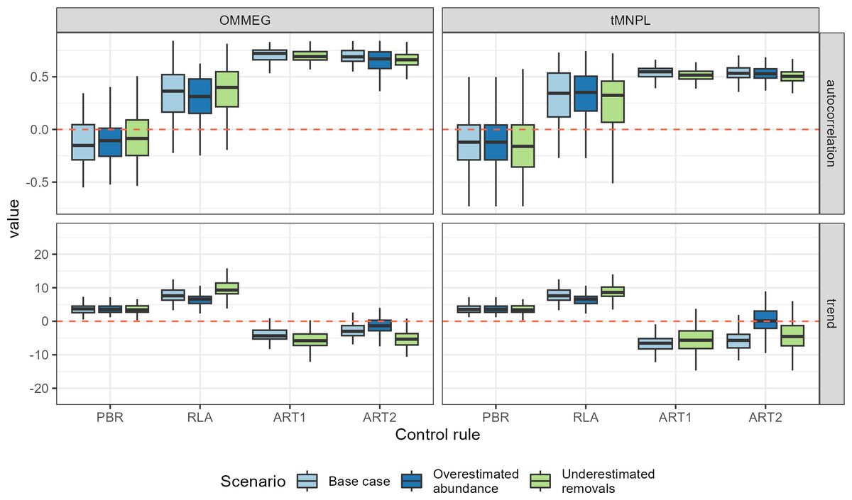
Figure 5: Performance metrics (continued).
Boxplots summarizing the distribution of autocorrelation (autocorrelation, unitless) and trend (trend, in % of previous limit). The red dashed line materializes the value 0.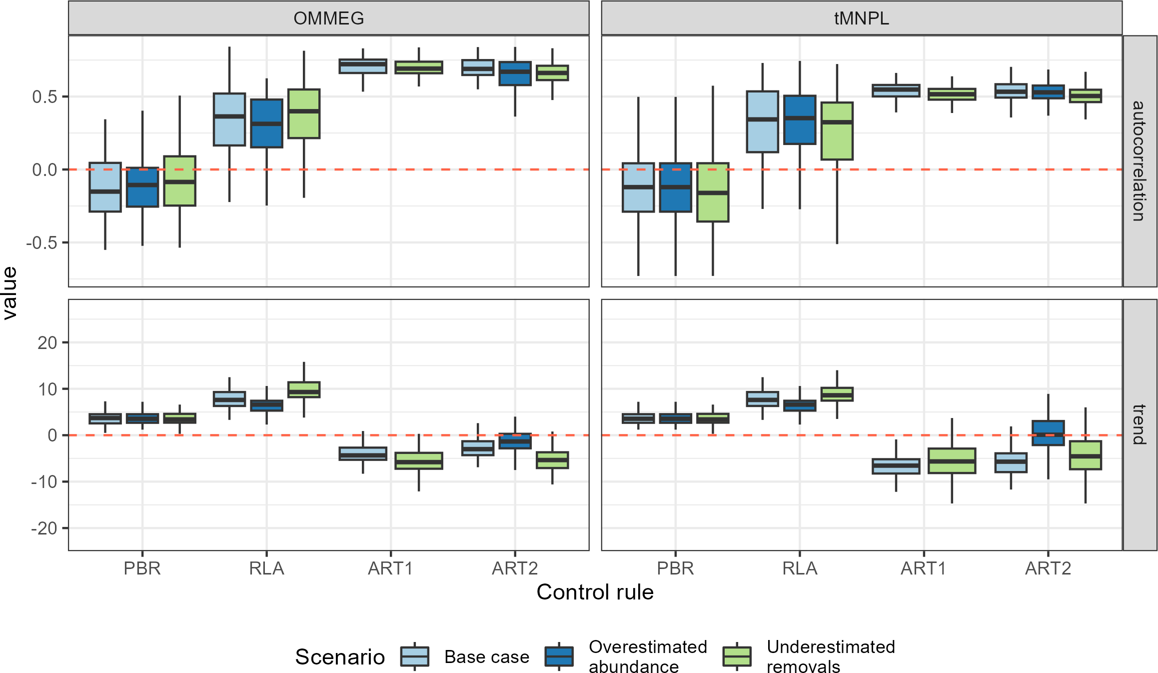
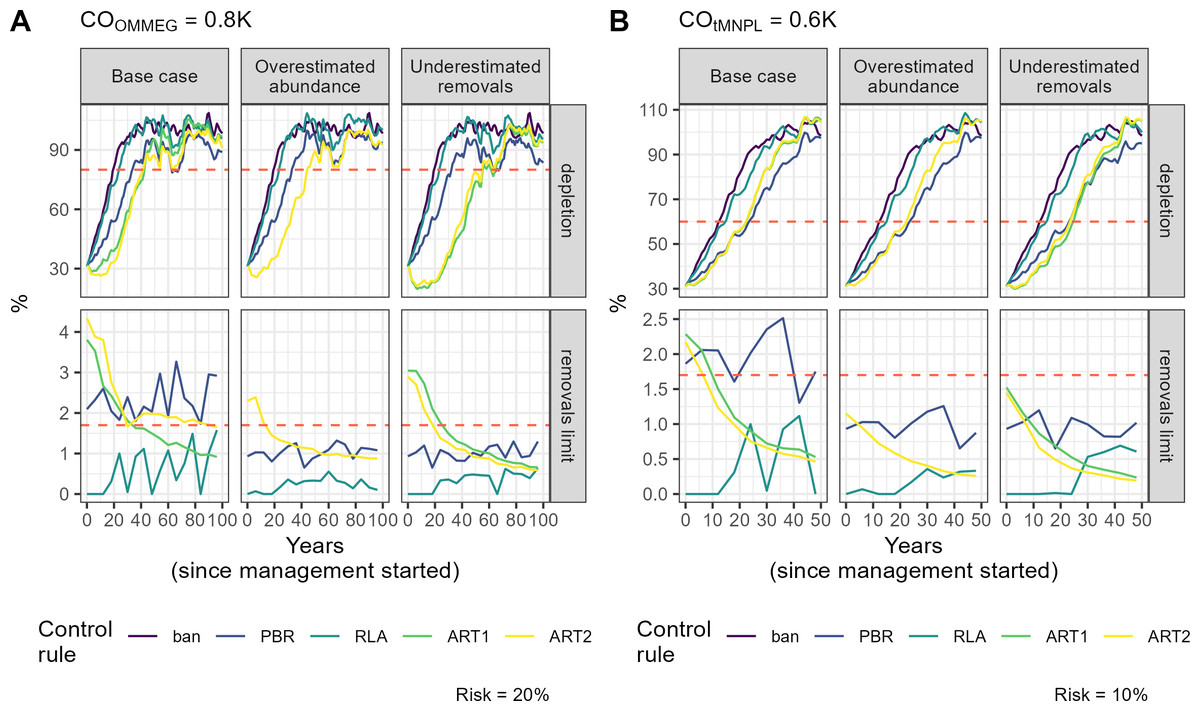
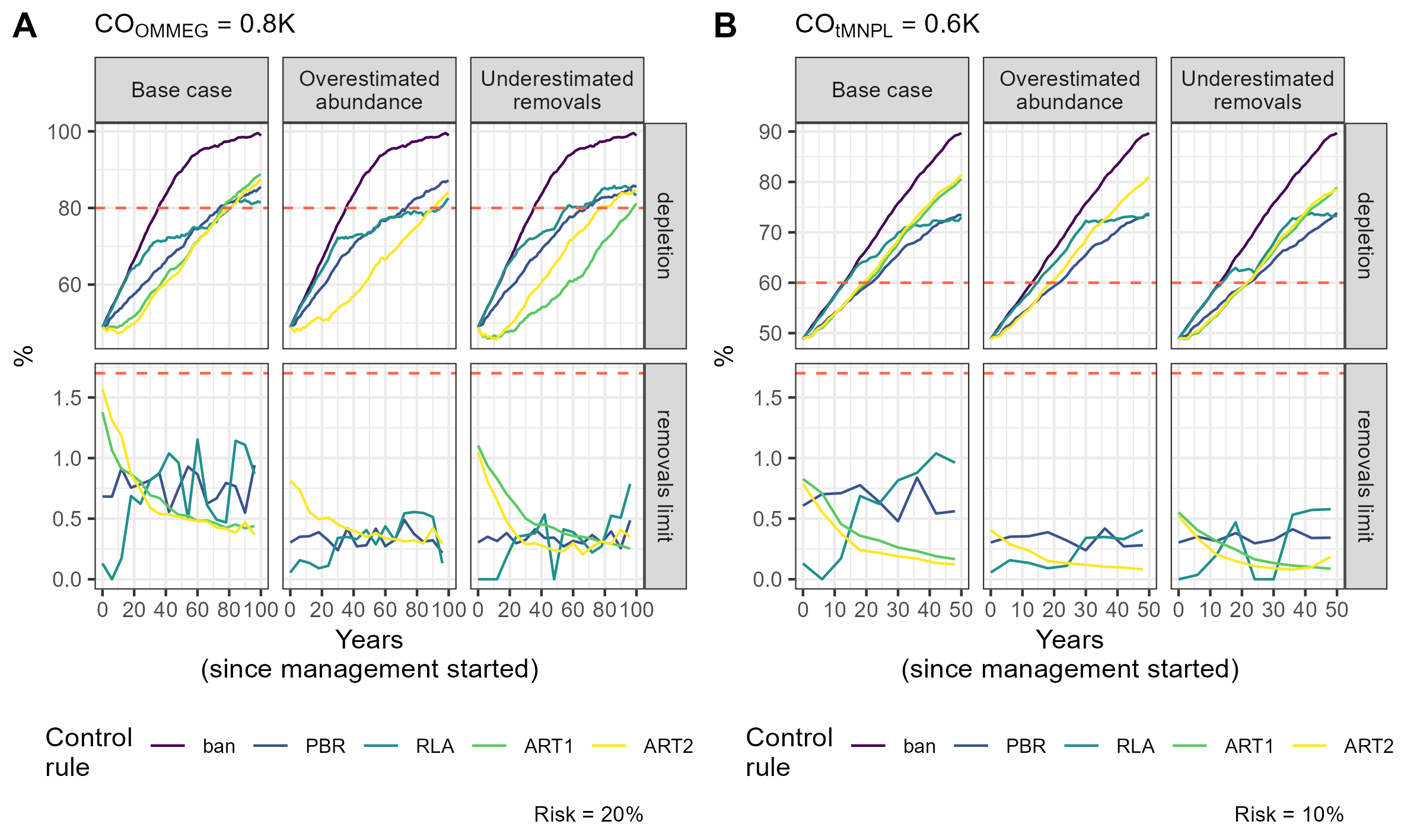
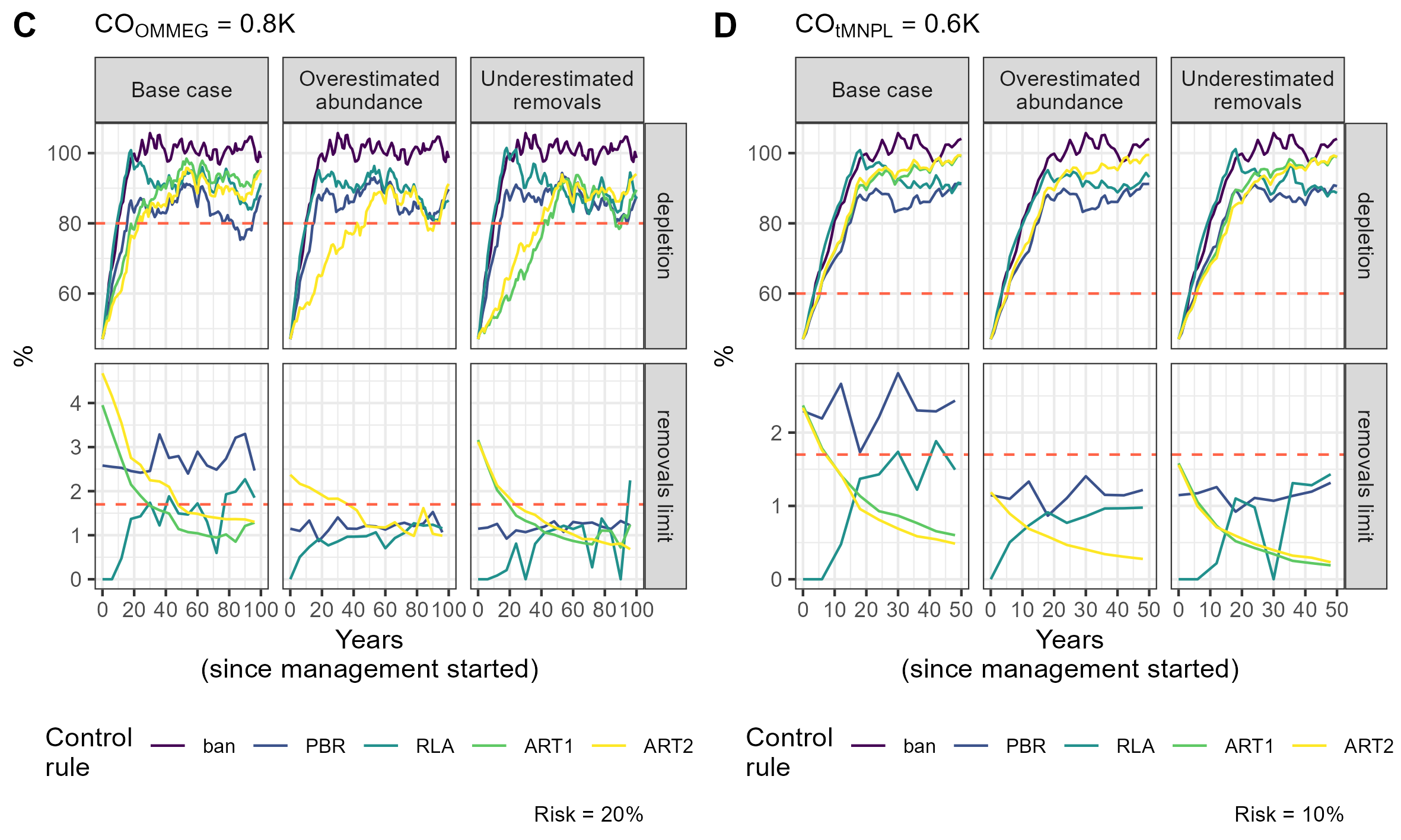
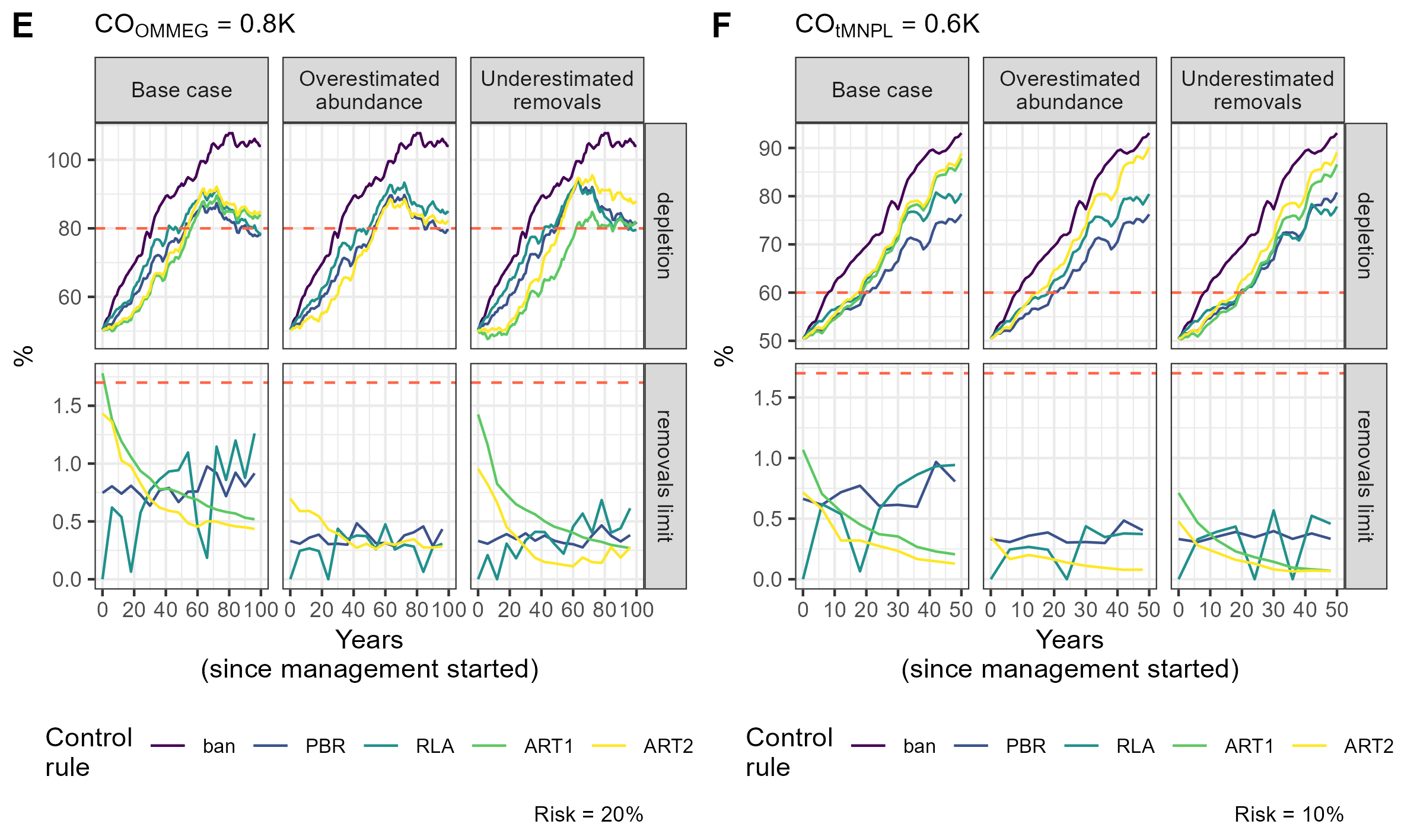
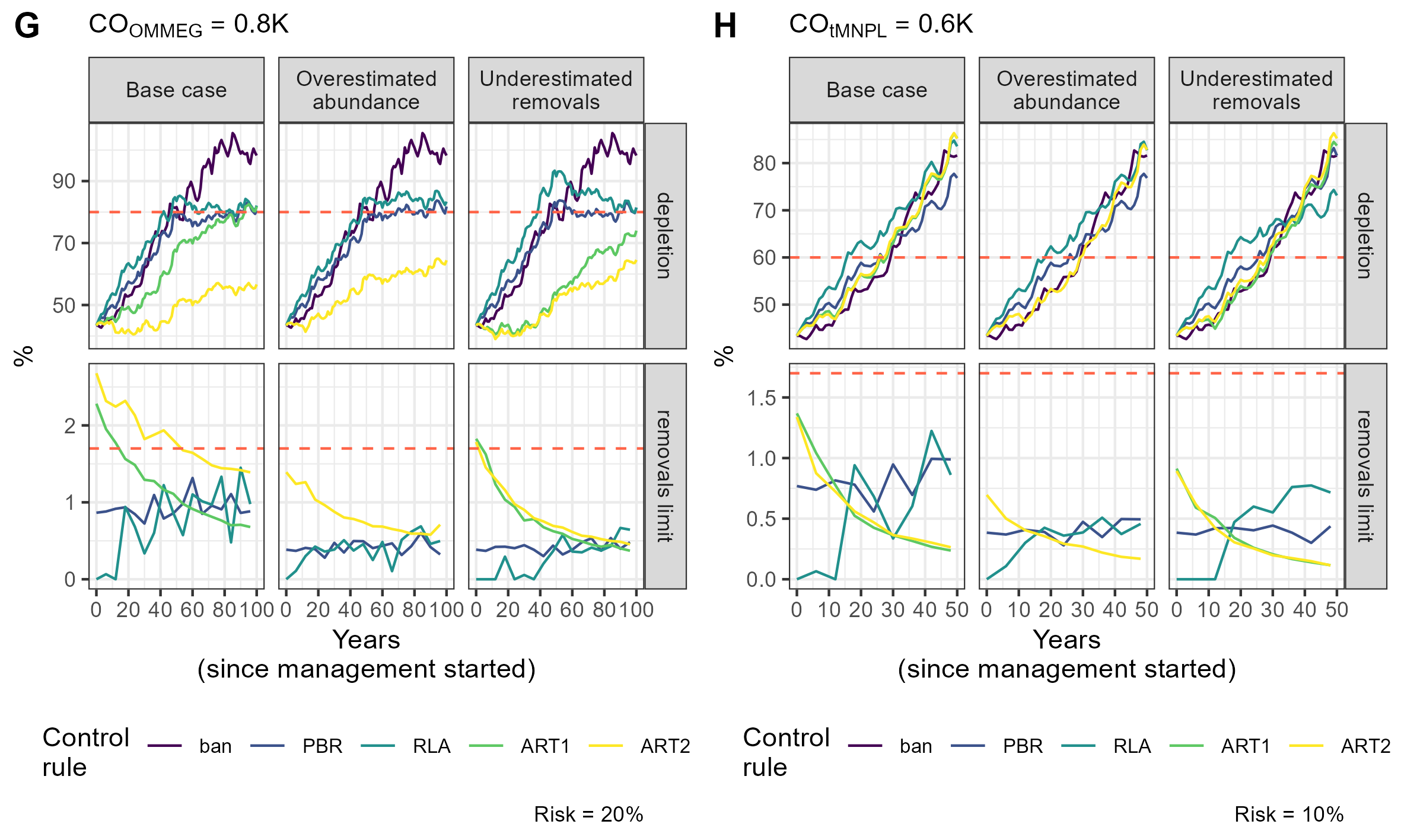
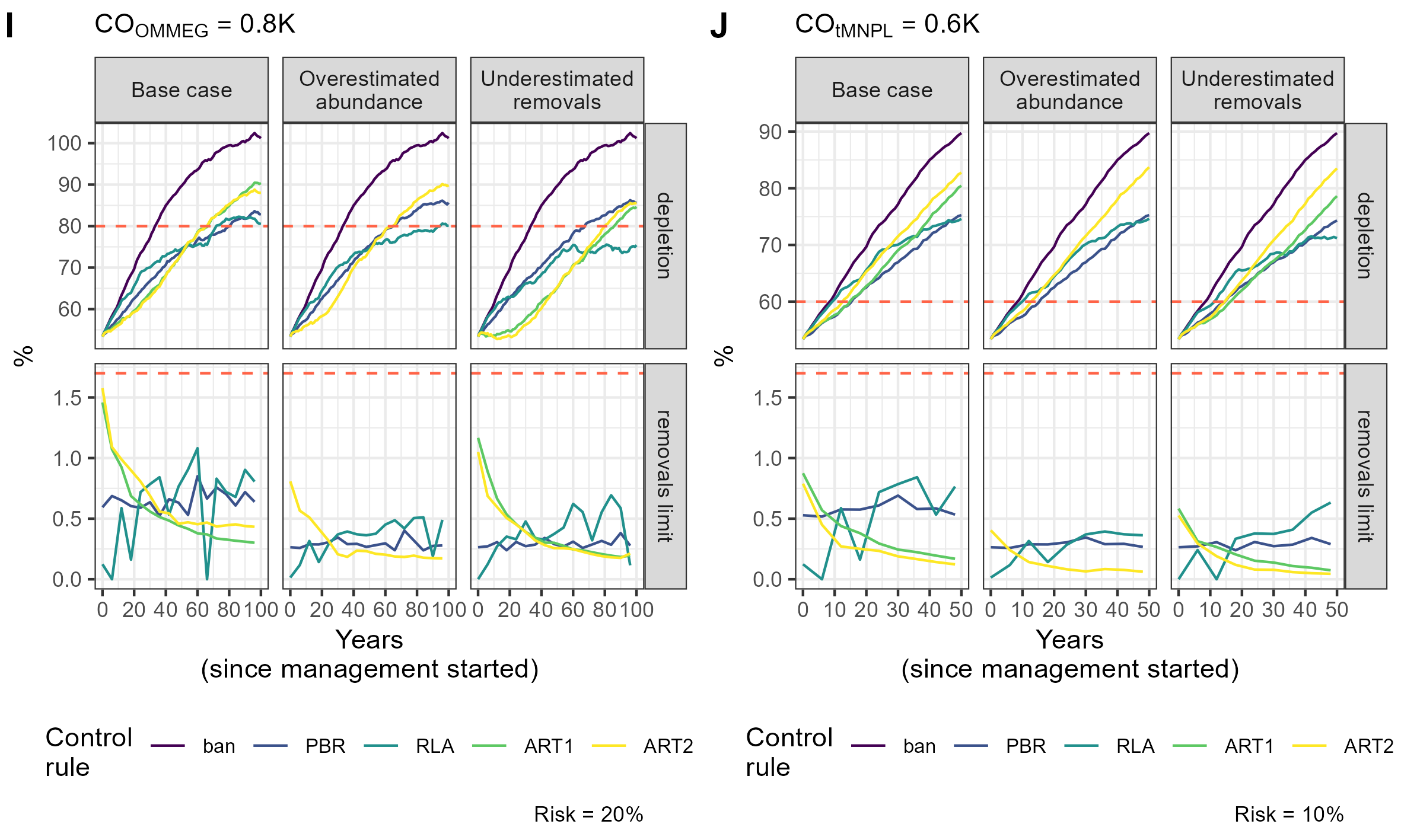
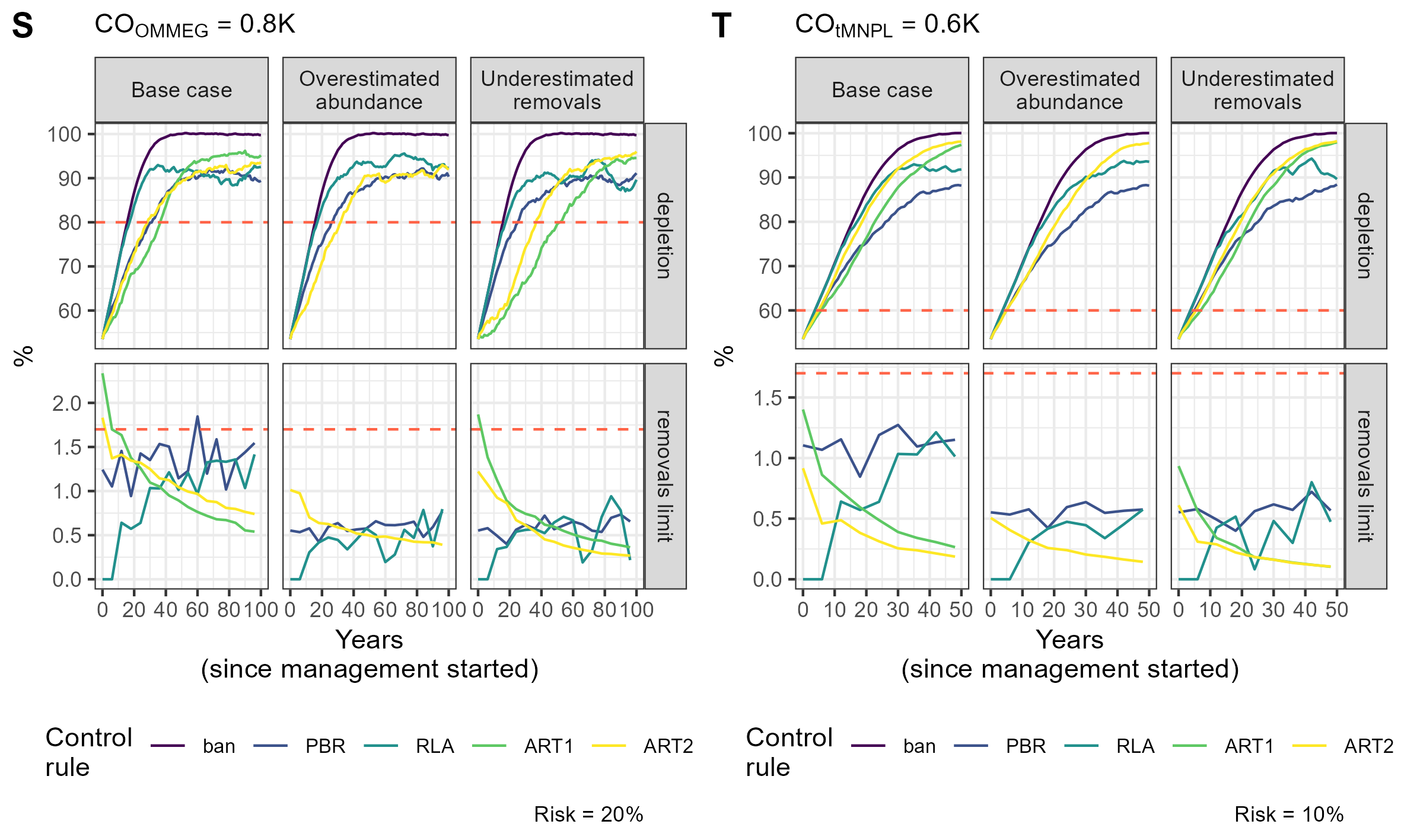
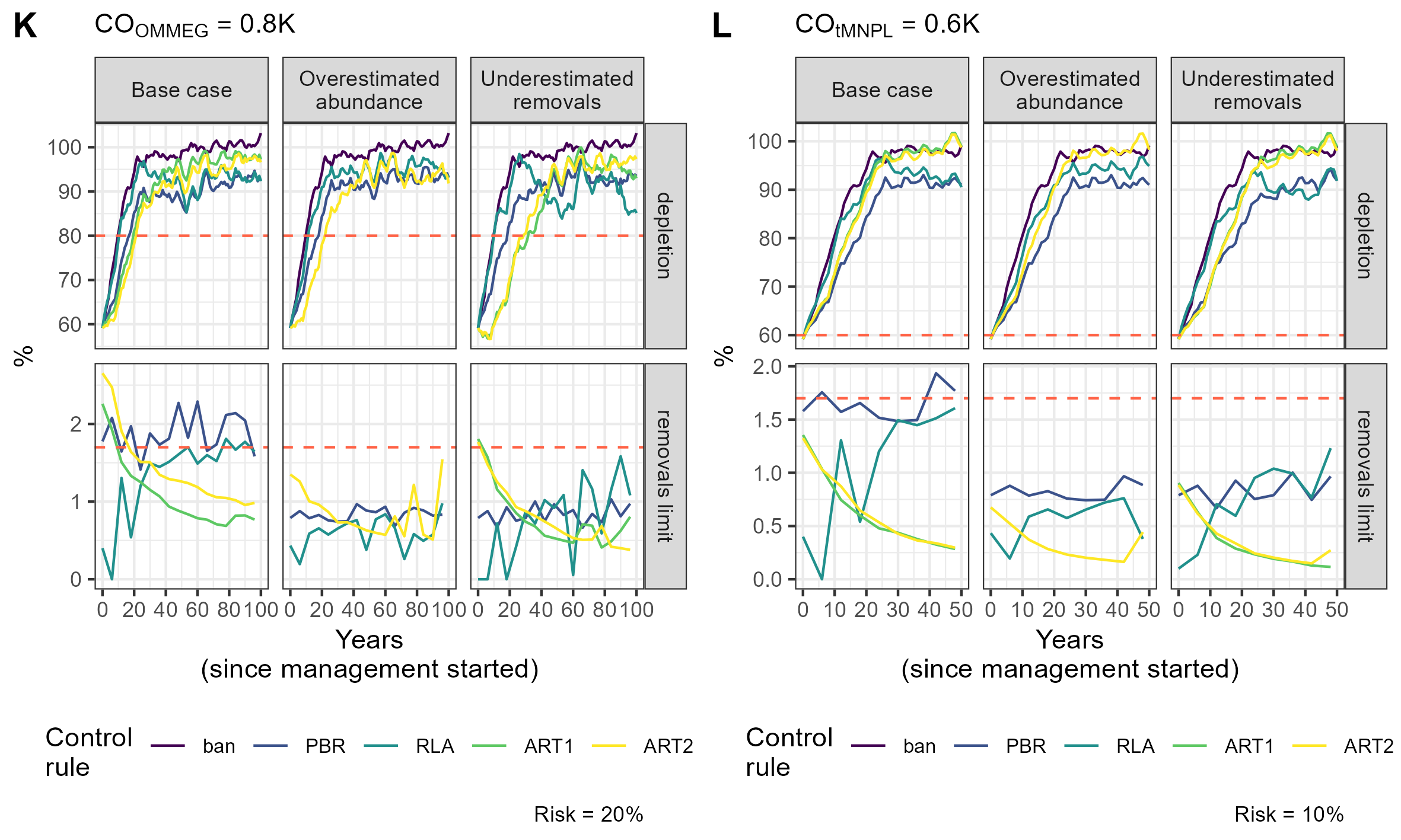
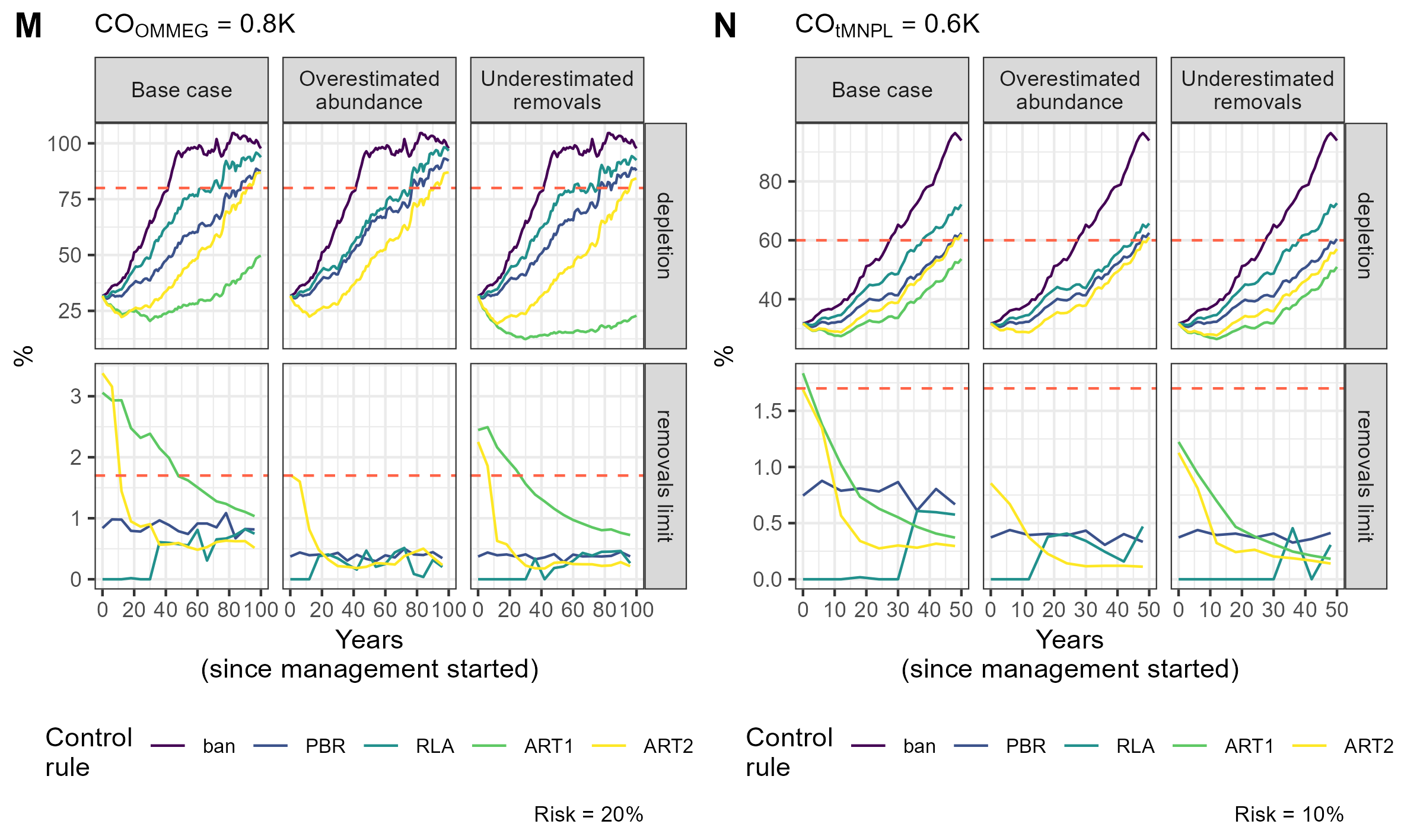
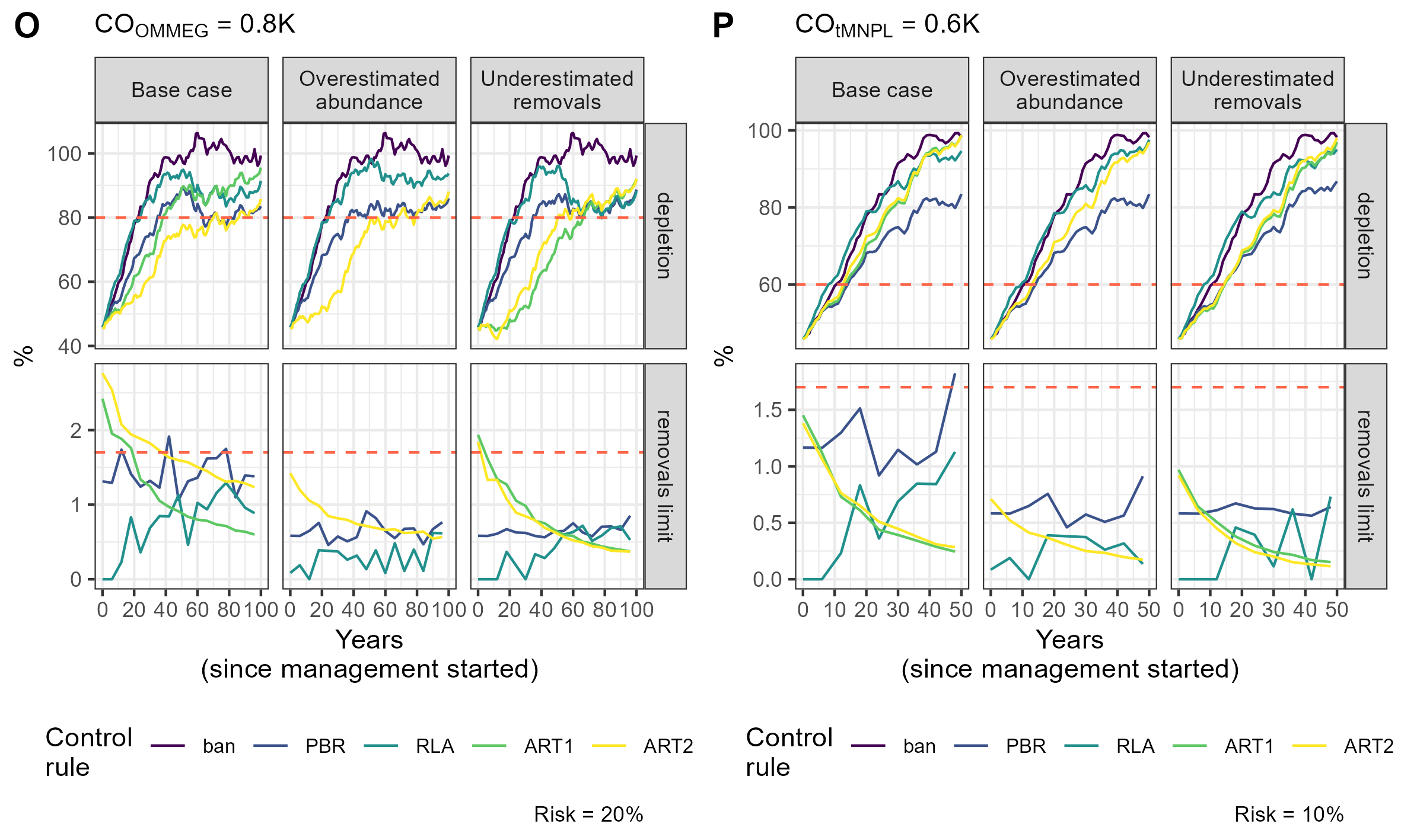
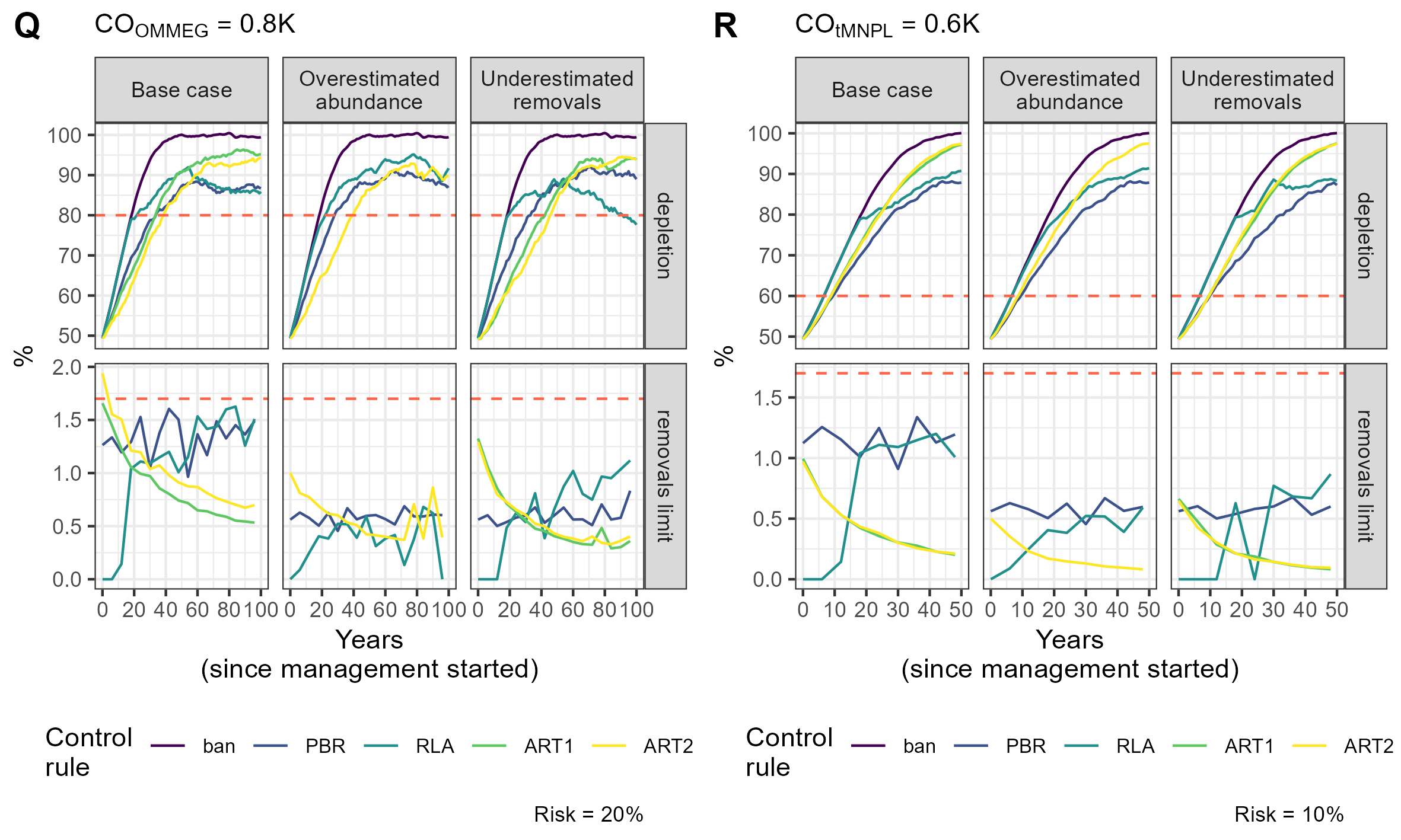
Figure 6: Example of a simulation.
Tuning with respect to the OMMEG interpretation of the ASCOBANS CO: to restore population to 80% of K with probability 0.8 in 100 years. (B) Tuning with respect to a CO of restoring population to a theoretical MNPL of 60% of K with probability 0.9 in 50 years. On the upper panel, the dashed red line materializes the depletion level targeted by the CO. On the lower panel, the dashed red line materializes the ASCOBANS fixed percentage of 1.7% (0.017) of the best available abundance estimate.
A Shiny application (Chang et al., 2022) for visualizing results is available at https://pelabox.univ-lr.fr/pelagis/DART/.
Discussion
We successfully developed candidate control rules for managing anthropogenic removals of PETS, a management imperative in a time of ever-expanding human activities in marine ecosystems (Intergovernmental Science-Policy Platform on Biodiversity and Ecosystem Services, 2018). These rules were rigorously tested in a MSE and benchmarked against other rules currently in use (e.g., Taylor et al. 2022) to investigate their properties and their potential for use in management. The candidate control rules ART rely on estimation of parameters from a newly developed stochastic SPM which are cornerstone of managing fisheries. All the rules tested, save for the fixed percentage and a candidate one (ART1), could be tuned to specific COs (Fig. 3).
The stochastic SPM herein developed abides by the ‘KISS’ principle (Zellner, 2002): ‘Keep It Sophistically Simple’. It does differ from the fixed percentage rule, which is only simple and not robust (Table 4), but not from the models underlying PBR or RLA (Punt, 2016; Genu et al., 2021). Where it does differ from the latter is in the number of parameters to estimate (Table 3) and in the explicit link made between the abundance process and removals (Eq. 6). The stochastic SPM views removals as a stochastic process whose variations reflect those of abundance. In contrast, the statistical models behind PBR or RLA are conditional on removals, which are not treated as stochastic but as a known covariate. The simplistic assumption of a time-invariant removal rate (that is, stationarity) made in the stochastic SPM is clearly wrong, and must be violated if management is to be effective: this rate is precisely the target of management, and measures should be taken to decrease it over time to align with current environmental aspirations in the North-East Atlantic. For instance, OSPAR endeavours with its North-East Atlantic Environment Strategy 2030 (Strategic Objective 7) to ensure that uses of the marine environment are sustainable, through the integrated management of current and emerging human activities. In particular, it aims at “minimis[ing] and if possible eliminat[ing] incidental by-catch of marine mammals, birds, turtles and fish so that it does not represent a threat to the protection and conservation of these species by 2030” (OSPAR, 2021).
Remarkably, the control rules that managed (on average) to decrease, and thereby minimise, the removal rate over time were ART1 and ART2 (Table 5, Fig. 6; see associated Shiny app (https://pelabox.univ-lr.fr/pelagis/DART/)). This feature was achieved thanks to a time-weighted likelihood approach in parameter estimation (Eq. (9)). Currently, the method for choosing weights in weighted likelihood is not formalized and is beyond the scope of this investigation. One potential venue is to consider a formal Decision Theory analysis for choosing a value for , for example using where pen(θ, η) is a penalty term for regularization to be made explicit in future work. In this study, an arbitrary choice for was used: this does not differ from the control rule RLA which also used a weighted likelihood and a weight that was found to work well in practice (Cooke, 1999; Boyce, 2000). In practice, the lack of robustness (Fig. 3) of candidate rule ART1 disqualifies it from further consideration and only ART2 remains competitive.
The control rule that was the most stable was PBR: it had the smallest variability (as gauged by the performance metrics cv; Table 5; see associated Shiny app (https://pelabox.univ-lr.fr/pelagis/DART/)). The value of the coefficient of variation was close to 23.5%, the mean value assumed for the precision of abundance estimates in the operating model (Fig. 2). This result was expected as the only source of variation in a limit set with PBR comes from the uncertainty in abundance estimates. This result merely testified to a correct implementation of functions in the package RLA (see Table 3 for the bespoken functions). The rule that had the most variability was RLA: this variability was borne out of the ability to set nill removals limits thanks to a feedback mechanism honing in on evidence of excessive depletion (the so-called Internal Protection Level, see Eq. (2)). The necessity of having nill limits stems from the tumultuous history of whaling management (e.g., Fitzmaurice, 2015) where, in a nutshell, the interplay of excessive quotas and over-investment in fleet capacity led to the systematic depletion of whale stocks. The RLA, a child of the IWC catch limit algorithm (see Internation Whaling Commission (2012) for a full description of the CLA), inherited this ability with an IPL currently set to 54% of K (Punt, 1993; Butterworth & Best, 1994), and displayed the shortest delays to recovery among the different tested rules (Table 5, Fig. 5). However, setting a limit to naught can be quite abrupt, resulting in non-smooth profile of removals limits over time and a high volatility. The latter presents clear challenges to the social acceptability of removals limits as a sudden ban on removals amounts to the cessation of fishing activities, leaving no room for a smoother transition of human activities towards reduced removals. In addition, the IPL represents another free parameter that can be challenged by stakeholders given its importance, and RLA could lead to ‘haggling’ and a displacement (sensu Rayner 2012) of the conservation issue of managing PETS removals towards a wild goose chase of endless simulation testing to identify, for example, an ‘optimal IPL’.
While the ability to set nill limits may be desirable from a conservation point of view, it may also entrench polarization between stakeholders vying for the attention of policy makers (see for example the discussion in Authier, Rouby & Macleod, 2021). Conservationists should, however, be aware that the RLA rule (and PBR to a lesser extent) also allows limits to increase over time as populations recover. This increase does not align with a desideratum to minimise, or when possible eliminate, anthropogenic removals of PETS: RLA is a double-edged sword that should be handled with care. In contrast, the candidate rule ART2 had a very different behaviour: its use resulted in a slow recovery because removals limits remained initially high, and sometimes above the ASCOBANS definition on ’unacceptable interactions’ (corresponding to 1.7%; Fig. 6 and Supplementary Information Appendix 5). There was also a high autocorrelation between successive limits set according to this rule (Table 5). These features can be assets for the acceptability of this rule in policy fora as it may favor gradual changes in practices that are at the root of removals, thereby giving time in finding mitigation actions or industry adaptations. The progressive decrease in removals limits makes it also clear that removals need to be minimized, as limits will be lowered progressively. This predictable behaviour is transparent to stakeholders who know before hand to expect each successive limit to be similar to the previous one, yet lower by ≈5% (in the current set of simulations; see Table 5).
One clear asset of the candidate rule ART2 is its built-in negative feedback of any evidence for a decline in abundance on removals limits. The trend estimated by the regularized approach has a low type-S (i.e., sign) error rate (Gelman & Tuerlinckx, 2000; Authier et al., 2020): this property explains the similarity between limits sets with or without taking this trend into account (Fig. 6). Authier et al. (2020) chose to estimate a trend that is relative to the first available abundance estimate. The rationale for this modelling choice stems from EU conservation instruments such as the HD which defines baselines as the abundance estimate at the time of enactment of the directive (1992), or the estimate closest to that date. The non-deterioration principle holds that management action should not lead to a worsening of conservation status over time, which is precisely what the candidate rule ART2 endeavours to achieve. However this rule does not forbid further degradation in the very short-term if unmanaged removals have been very high as recent past removal rates inform heavily this rule (see Fig. 6). In the EU, the current overaching conservation instrument for marine ecosystems is the MSFD. Its biodiversity indicator is built on several criteria including by-catch (non-intentional removals due to fisheries) and population abundance. A recent assessment of the abundance of cetaceans at the level of the North-East Atlantic for OSPAR’s Quality Status Report 2023 was based on estimation of such trends (Geelhoed et al., 2022). The candidate rule ART2 meshes together abundance indicators and removals limits, and has thereby the potential to achieve a seamless integration of current regional indicators (Geelhoed et al., 2022; Taylor et al., 2022), at least for cetaceans. This meshing resulted in increased robustness: in the scenario where abundance was overestimated, the recovery factor for ART2 was not reduced and remained the same as in the base case scenario (Fig. 3).
Our investigation and benchmarking of several control rules was carried out assuming a single stock or population for the PETS of interest. This assumption translates as a closed population with no migration, either in or out of the area of interest. This choice stems partly from simplicity considerations, and from familiarity with some wide-ranging cetacean species with one single assessment unit in the North-East Atlantic (e.g., the common dolphin Geelhoed et al., 2022). Venues for future work are developing multi-stock operating models to further assess the robustness of control rules against uncertainty in stock/population structure (Hammond & Donovan, 2003). Such developments will be undertaken for integration in the RLA package (Genu et al., 2021) and for carrying out MSE of increased ecological realism by considering scenarios with migration between source and sink populations when relevant. Finally, our focus on cetaceans is not prescriptive: the new control rule could be tested in an MSE framework for other taxa (seabirds, sharks, etc.) with appropriate operating population dynamics models (Haider et al., 2017; Horswill, O’Brien & Robinson, 2017; Tsai, Liu & Chang, 2020; Tinker et al., 2022).
We envision that the control rule ART (and more precisely ART2 since ART1 is not robust) can be put to use in the current context of managing human activities in the Northeast Atlantic (McQuatters-Gollop et al., 2022), and more precisely to set thresholds on anthropogenic removals to assess by-catch (see e.g., Taylor et al., 2022). Managing PETS by-catch is fraught with many hurdles including the allocation problem (Holmes & Miller, 2022). In other words, once a threshold is known, how to divide it up between the different fisheries flying different flags? There are currently, to the best of our knowledge, no forum in the EU where this allocation issue is being discussed for PETS. One reason might be that the first step, assessing quantitatively the impact of anthropogenic activities at relevant ecosystemic scales is still in its infancy, and the recently OSPAR Quality Status Report for 2023 (https://oap.ospar.org/en/ospar-assessments/quality-status-reports/qsr-2023/) is a major step forward. Methodologies for setting thresholds are critical (Palialexis et al., 2021) and MSE are state-of-the-art in this respect (Rademeyer, Plagányi & Butterworth, 2007; Bunnefeld, Hoshino & Milner-Gulland, 2011; Punt et al., 2016; Kaplan et al., 2021). Focusing on marine mammals, PBR, RLA and ART can be calibrated to specific conservation objectives (a.k.a. “conceptual objectives” in Punt et al., 2016). The output of these control rules is a threshold, that is a value of PETS that can be removed each year within a MSFD cycle and with a policy-agreed-upon risk. This threshold corresponds to a management objective (a.k.a. “operational objectives” in Punt et al., 2016). It is important to keep in mind that PBR, RLA and ART are meant to be updated with new data on abundance and removals: as such the values they give are expected to change over time. In this (desk) MSE, we have devised a new control rule which can be updated every six years (corresponding to a MSFD cycle) for assessing anthropogenic removals. In particular, ART is a competitive control rule for developing threshold values for the maximum allowable mortality rate from incidental catches of PETS.
How to enforce relevant management actions that will ensure that these values are not exceeded remain the difficult question which we have not discussed here. This question is beyond the scope our this study, as it entails to tackle issues which are under the competence of the EU fishery common policy or EU member states, such as the allocation problem4 and the effective monitoring of fisheries.
Conclusion
After developing a stochastic SPM, we carried out an MSE to test two new candidate control rules for managing anthropogenic removals of marine PETS. One of these rules (ART1) turned out to be brittle but the other (ART2) was robust to plausible biases in data that can be typically collected on marine PETS. Our investigation was inspired by cetaceans, with which we are most familiar and which are impacted by anthropogenic activities (Taylor et al., 2022). Our results need not, however, be restricted to this taxonomic group. In particular, we identified a promising new control rule to minimize removals over time. This candidate rule not only compared favorably against rules currently in use to assess marine mammal removals, but displayed also greater alignment with EU conservation instruments and aspirations. One co-lateral result of our MSE, which tested two conservation objectives, is to highlight the remarkable effectiveness of the rule PBR in meeting CO rapidly. The light data requirements of PBR (Table 3) underscore how crucial are abundance estimates for managing PETS removals, and stress the need to secure adequate governance for monitoring schemes with adequate coverage for management purposes. For cetaceans, depending on species and current knowledge on population structure, several surveys provide important data in the North-East Atlantic (Geelhoed et al., 2022). A prominent example is the large-scale SCANS surveys in the North-East Atlantic (Hammond et al., 2013; Hammond et al., 2021b; Gilles et al., 2023). Estimates of human-induced removals of PETS are clearly needed (Murphy, Borges & Tasker, 2022), at the very least to be able to carry out assessments; and efforts to (i) make the best use of currently available data (Authier, Rouby & Macleod, 2021), or (ii) to develop data acquisition with Remote Electronic Monitoring (Kindt-Larsen et al., 2023) need to be pursued. Yet, this should not eclipse the need for regionally coherent, dedicated surveys (see e.g., Hammond et al., 2021a) that collect high-quality data to inform on PETS abundance (Gilles et al., 2023).
Decision-making usually involves trade-offs (Regan et al., 2005; Cressie, 2022). In this analysis, we investigated some of the salient trade-offs needed to move forward on managing the impacts of human activities in the North-East Atlantic (McQuatters-Gollop et al., 2022). We developed a stochastic SPM, whose full study is beyond the scope of this paper (Ouzoulias, 2022), and identified a promising candidate control rule for managing anthropogenic removals of marine PETS in an age of ever-expanding anthropic activities in the oceans.
Supplemental Information
Scripts to run the Management Strategy Evaluation (includes a shiny app. and an R package)
Performance metrics (log scale)
Boxplots summarizing the distribution of variability (cv, unitless), mean (average, as a proportion of current abundance estimate; e.g., 0.01 = 1 %), and delay in recovery (in years). The y-axis is on a logarithmic scale.
Simulation example 1
Example of simulations: 10 simulations within MSE on assessing PETS long-term viability.
Simulation example 2
Example of simulations: 10 simulations within MSE on assessing PETS long-term viability.
Simulation example 3
Example of simulations: 10 simulations within MSE on assessing PETS long-term viability.
Simulation example 4
Example of simulations: 10 simulations within MSE on assessing PETS long-term viability.
Simulation example 5
Example of simulations: 10 simulations within MSE on assessing PETS long-term viability.
Simulation example 6
Example of simulations: 10 simulations within MSE on assessing PETS long-term viability.
Simulation example 7
Example of simulations: 10 simulations within MSE on assessing PETS long-term viability.
Simulation example 8
Example of simulations: 10 simulations within MSE on assessing PETS long-term viability.
Simulation example 9
Example of simulations: 10 simulations within MSE on assessing PETS long-term viability.
Simulation example 10
Example of simulations: 10 simulations within MSE on assessing PETS long-term viability.