
Common laboratory results-based artificial intelligence analysis achieves accurate classification of plasma cell dyscrasias
- Published
- Accepted
- Received
- Academic Editor
- Vladimir Uversky
- Subject Areas
- Computational Biology, Hematology, Oncology, Computational Science, Data Mining and Machine Learning
- Keywords
- Artificial intelligence, Machine learning, Plasma cell dyscrasias, Diagnosis, Classification, Laboratory biomarkers
- Copyright
- © 2024 Yao et al.
- Licence
- This is an open access article distributed under the terms of the Creative Commons Attribution License, which permits using, remixing, and building upon the work non-commercially, as long as it is properly attributed. For attribution, the original author(s), title, publication source (PeerJ) and either DOI or URL of the article must be cited.
- Cite this article
- 2024. Common laboratory results-based artificial intelligence analysis achieves accurate classification of plasma cell dyscrasias. PeerJ 12:e18391 https://doi.org/10.7717/peerj.18391
Abstract
Background
Plasma cell dyscrasias encompass a diverse set of disorders, where early and precise diagnosis is essential for optimizing patient outcomes. Despite advancements, current diagnostic methodologies remain underutilized in applying artificial intelligence (AI) to routine laboratory data. This study seeks to construct an AI-driven model leveraging standard laboratory parameters to enhance diagnostic accuracy and classification efficiency in plasma cell dyscrasias.
Methods
Data from 1,188 participants (609 with plasma cell dyscrasias and 579 controls) collected between 2018 and 2023 were analyzed. Initial variable selection employed Kruskal-Wallis and Wilcoxon tests, followed by dimensionality reduction and variable prioritization using the Shapley Additive Explanations (SHAP) approach. Nine pivotal variables were identified, including hemoglobin (HGB), serum creatinine, and β2-microglobulin. Utilizing these, four machine learning models (gradient boosting decision tree (GBDT), support vector machine (SVM), deep neural network (DNN), and decision tree (DT) were developed and evaluated, with performance metrics such as accuracy, recall, and area under the curve (AUC) assessed through 5-fold cross-validation. A subtype classification model was also developed, analyzing data from 380 cases to classify disorders such as multiple myeloma (MM) and monoclonal gammopathy of undetermined significance (MGUS).
Results
1. Variable selection: The SHAP method pinpointed nine critical variables, including hemoglobin (HGB), serum creatinine, erythrocyte sedimentation rate (ESR), and β2-microglobulin. 2. Diagnostic model performance: The GBDT model exhibited superior diagnostic performance for plasma cell dyscrasias, achieving 93.5% accuracy, 98.1% recall, and an AUC of 0.987. External validation reinforced its robustness, with 100% accuracy and an F1 score of 98.5%. 3. Subtype Classification: The DNN model excelled in classifying multiple myeloma, MGUS, and light-chain myeloma, demonstrating sensitivity and specificity above 90% across all subtypes.
Conclusions
AI models based on routine laboratory results significantly enhance the precision of diagnosing and classifying plasma cell dyscrasias, presenting a promising avenue for early detection and individualized treatment strategies.
Introduction
The 2022 International Consensus Classification (ICC) identifies plasma cell neoplasms, including multiple myeloma (MM), monoclonal gammopathy of undetermined significance (MGUS), solitary plasmacytoma (SBP), light-chain amyloidosis (AL), and lymphoplasmacytic lymphoma (LPL), as a continuum of related disorders (Fend, Dogan & Cook, 2023). However, overlapping clinical markers and variable risks of disease progression present significant challenges for traditional diagnostic approaches (Brigle & Rogers, 2017). Current methods rely heavily on the CRAB criteria (hypercalcemia, renal insufficiency, anemia, and bone lesions) and tumor burden (Rajkumar et al., 2014; Kuehl & Bergsagel, 2002; Kyle et al., 2010; Landgren et al., 2009), which frequently fail to distinguish between precursor conditions and malignant stages, leading to delayed interventions or misdiagnosis, with serious consequences for patient outcomes (Schinke et al., 2020). For instance, MM is defined by clonal plasma cell proliferation within the bone marrow, resulting in skeletal degradation and eventual collapse (Cowan et al., 2022). Representing approximately 1.8% of all malignancies and over 15% of hematologic cancers in the U.S., MM poses a substantial clinical burden (Cerchione & Martinelli, 2020; Firth, 2019). Studies reveal that diagnostic pathways for MM are intricate, and later-stage diagnoses correlate with increased recurrence rates and diminished survival (Kazandjian, 2016), underscoring the necessity to reassess conventional diagnostic and monitoring strategies (Kumar et al., 2020).
Artificial intelligence (AI), particularly machine learning models, offers a transformative solution to these diagnostic limitations (Allegra et al., 2022). AI’s ability to process routine laboratory data and detect subtle patterns that elude traditional methods significantly enhances the speed and precision of early detection (Rabbani et al., 2022). This study developed AI-driven models using gradient-boosted decision trees (GBDT) (Li et al., 2020) for diagnosis and deep neural networks (DNN) for subtype classification, leveraging critical laboratory variables to enable accurate and efficient classification of plasma cell dyscrasias.
Materials and Methods
Patients and methods
The study adhered to the principles of the Declaration of Helsinki and received approval from the Medical Ethics Committee of Zhejiang Provincial People’s Hospital (Approval No. Zhejiang Provincial People’s Hospital Ethics 2024 Other No. 034, Acceptance No. QT2024029). Given the retrospective design, the Ethics Committee granted a waiver for the requirement of individual informed consent.
Patients and data selection
A retrospective analysis was conducted on common and biochemical markers from 609 newly diagnosed plasma cell dyscrasia cases and 579 control cases (comprising infectious diseases, autoimmune disorders, liver diseases, and kidney diseases) treated at Zhejiang Provincial People’s Hospital between January 2018 and February 2024. To further evaluate the model’s clinical applicability and generalizability, data from an additional 30 newly diagnosed plasma cell dyscrasia cases and 34 control cases were included. Diagnoses followed the 2014 International Myeloma Working Group (IMWG) criteria. Thirteen variables—sex, age, hemoglobin (HGB), calcium, serum creatinine, erythrocyte sedimentation rate (ESR), κ light chain, λ light chain, κ/λ ratio, albumin/globulin ratio, albumin, globulin, and β2-microglobulin—were selected as initial modeling variables, representing key biomarkers associated with the CRAB criteria. These markers have been validated as independent diagnostic indicators for plasma cell dyscrasias (Cowan et al., 2022), aiding in early detection. For subtype classification, additional data on immunofixation electrophoresis and CD markers were utilized. A deep learning model was employed, optimizing classification accuracy and effectively distinguishing between plasma cell dyscrasia subtypes.
Despite the essential role of radiological assessments, such as X-ray, whole-body MRI, and PET-CT, in diagnosing plasma cell dyscrasias, these modalities were deliberately excluded from the analysis. The focus was on developing a model based solely on routine laboratory parameters, which are more accessible and cost-effective, allowing for broader and faster clinical implementation. Incorporating radiological data could introduce variability due to differing resource availability, potentially compromising model performance. The emphasis on routine laboratory markers aimed to preserve simplicity and clinical practicality, though it is acknowledged that the exclusion of radiological data may limit the model’s ability to capture certain disease-specific features.
Methodology for evaluating different variables
Demographic and clinical parameters: Sex and age were documented at the time of diagnosis.
Biochemical marker evaluation: HGB, calcium ions (Ca2+), serum creatinine, ESR, κ and λ light chains, albumin, globulin, and β2-microglobulin were quantified using standard clinical laboratory techniques. Automated analyzers were utilized for HGB and calcium measurements, nephelometry for light chain assessment, and ELISA for β2-microglobulin detection.
Flow cytometry (MFC) analysis: Multiparametric flow cytometry (MFC) was employed to assess CD markers, including CD45, CD38, and CD138, using an antibody panel with 8–12 fluorochromes. Antigen expression was classified as positive when more than 10% of plasma cells demonstrated expression. Table S1 provides detailed antibody-fluorochrome combinations, and further information on tube combinations is available in Table S2.
Data processing
Based on diagnostic criteria and physicians’ auxiliary judgments, factors relevant to diagnosing plasma cell dyscrasias were identified. Raw data for diagnostic prediction were extracted from the LIS database, but the initial dataset required additional preprocessing before it could be used to train machine learning algorithms.
Missing value handling
A significant portion of missing values, especially in immunoglobulin and immunophenotyping data, was observed among non-plasma cell dyscrasia patients. As immunophenotyping and immunoglobulin tests could influence the model, two corresponding data columns were removed. Missing values were predominantly found in the ESR and β2-microglobulin features, which were handled using mean imputation—replacing missing values with the feature’s average. For categorical features, mode imputation was applied. In addition to these imputation techniques, attention-based deep learning algorithms were used to encode different features. Missing values were labeled as exceptional and masked to enable distinct feature encoding, preserving more information compared to conventional imputation methods.
Categorical feature processing
Machine learning and deep learning models require numerical input features. Therefore, categorical variables were converted into numerical formats. A direct numerical assignment approach was avoided for immunofixation electrophoresis, as this could introduce misleading intensity information. Instead, one-hot encoding (Zhu, Qiu & Fu, 2024) was applied, breaking immunofixation electrophoresis into five binary columns: G, A, M, κ, and λ. Each column was represented as a binary value, where 0 indicated a negative result and one indicated a positive one, converting immunofixation electrophoresis data into a 5-dimensional binary vector.
Variable selection
To develop a robust classification system and identify key laboratory variables specific to plasma cell dyscrasias, a systematic analysis was conducted, comparing data between plasma cell dyscrasias and non-plasma cell dyscrasias. The Kruskal-Wallis (K-W) test or Wilcoxon rank-sum test, along with multiple logistic regression, were employed to evaluate the differential expression of laboratory variables between the two groups. Forest plots were used for visual comparison. Through final dimensionality reduction, nine critical variables were identified for the diagnostic model: HGB, age, serum creatinine, ESR, κ/λ light chain ratio, κ light chain, λ light chain, globulin, and β2-microglobulin. All statistical tests were considered significant at p < 0.05 (two-tailed).
Patient characteristics
This study focuses on classifying plasma cell dyscrasias and non-plasma cell dyscrasias to develop predictive diagnostic models. A comparative analysis of clinical features and outcomes between individuals with plasma cell dyscrasias and non-plasma cell dyscrasias in the derived cohort is presented in Table 1. Over the study period, 1,188 patients were divided into training and internal validation sets, while an external group of 64 patients was used for validation.
| Variables | Plasma cell dyscrasias (n = 609) |
Non-plasma cell dyscrasias (n = 579) |
P |
|---|---|---|---|
| Sex (female/male) | 223/386 (37%/63%) | 235/344 (41%/59%) | p = 0.562 |
| Age (year) | 69 (60, 76) | 59 (48, 71) | P < 0.0001 |
| Hemoglobin (g/L) | 97.82 (25.82) | 120 (105, 140) | P < 0.0001 |
| Serum calcium (mmol/L) | 2.22 (2.08, 2.34) | 2.23 (2.11, 2.34) | p = 0.11 |
| Serum creatinine (μmol/L) | 87.30 (67.70, 135.5) | 99.10 (73.80, 180.20) | P < 0.0001 |
| ESR (mm/h) | 40 (25, 67) | 17 (10, 30) | P < 0.0001 |
| Light chain κ/λ ratio | 2.67 (0.20, 8.70) | 1.50 (0.92, 1.93) | P < 0.0001 |
| Light chain κ (g/L) | 60.10 (11.10, 420.00) | 14.50 (9.30, 37.05) | P < 0.0001 |
| Light chain λ (g/L) | 35.00 (7.00, 300.00) | 11.35 (5.40, 30.50) | P < 0.0001 |
| Albumin/globulin ratio | 1.01 (0.61, 1.48) | 1.31 (1.11, 1.53) | P < 0.0001 |
| Albumin (g/L) | 33.25 (28.00, 37.60) | 36.80 (31.60, 40.48) | P < 0.0001 |
| Globulin (g/L) | 32.60 (24.38, 51.80) | 27.50 (23.90, 31.18) | P < 0.0001 |
| β2-macroglobulin (mg/L) | 4.50 (3.01, 7.48) | 1.90 (0.39, 4.50) | P < 0.0001 |
Diagnostic model development
Given the model’s diagnostic and classification capabilities, gradient boosting decision trees (GBDT) are recognized as a highly effective ensemble learning method (Hastie et al., 2009). As a commonly used algorithm in ensemble learning, GBDT was implemented to predict whether patients are affected by plasma cell disorders. GBDT is a boosting-based technique designed for tabular prediction tasks, and it operates as an additive model consisting of multiple CART decision regression trees. The model works by iteratively constructing decision trees, where k represents the number of trees, and denotes the output of the i-th regression tree. In binary classification, is selected based on the mean squared error (MSE) between and the labels as the loss function L. The negative gradient of the total loss J is calculated to fit each successive regression tree (x), and these trees are ultimately combined to generate the final prediction.
(1)
(2)
The maximum number of regression trees was set to 100, with a minimum leaf size of 2 and a learning rate of 0.1. Preprocessing steps included data imputation, cleaning, and encoding of categorical features. Parameter tuning was performed using 5-fold cross-validation. For external validation, 30 newly diagnosed plasma cell dyscrasias cases and 34 non-plasma cell dyscrasias cases were selected. The GBDT classifier, trained on the original dataset, demonstrated strong generalization, proving both clinically practical and applicable. The full training pipeline is illustrated in Fig. 1.
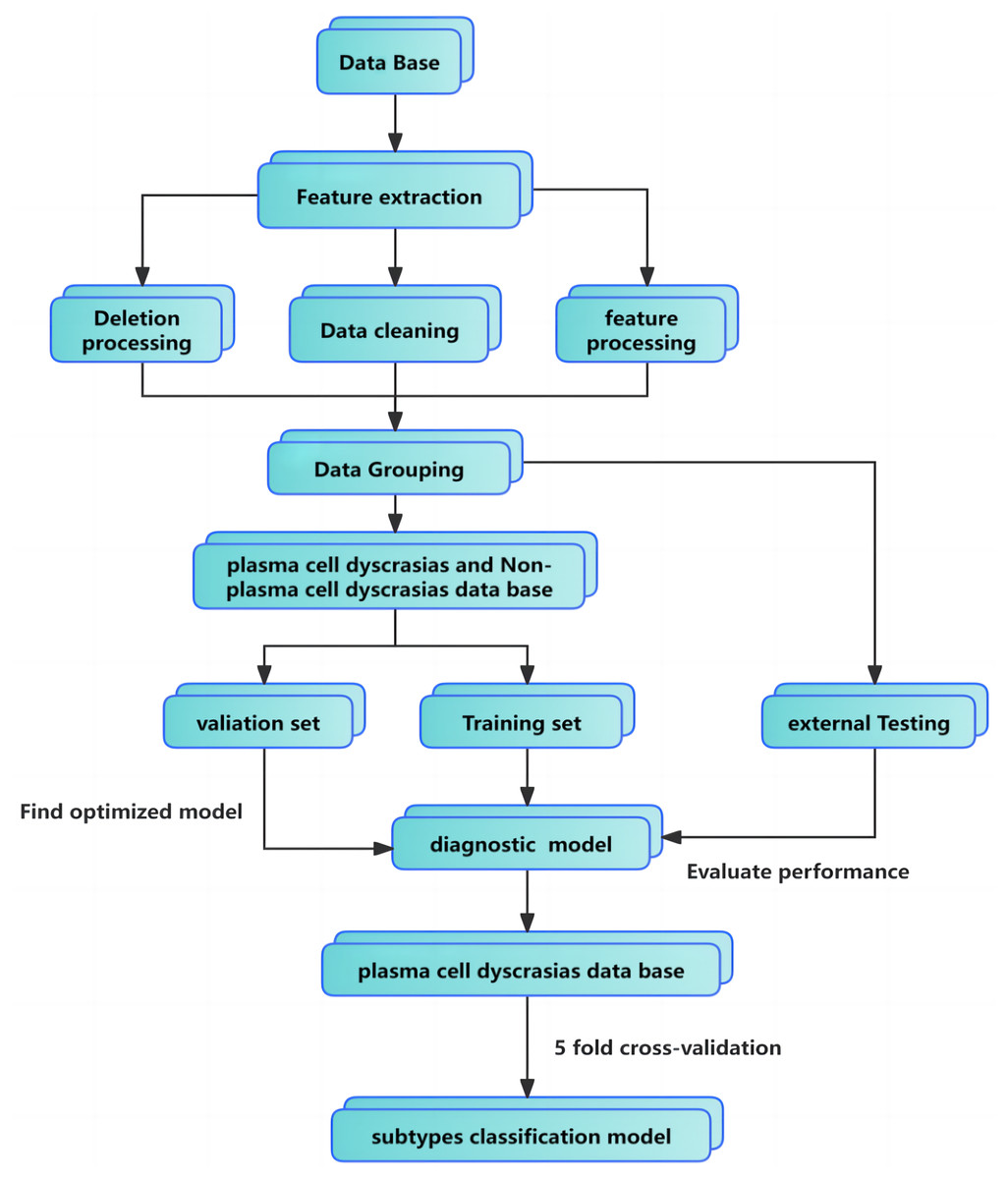
Figure 1: Classification model flowchart and training pipeline.
Performance evaluations were also conducted by comparing the GBDT model with support vector machines (SVM) (Rabbani et al., 2022), deep neural networks (DNN) (Li et al., 2020), and decision trees (DT). The SVM model was designed to identify the hyperplane that maximizes the margin in feature space. A penalty coefficient of one was selected, and the Gaussian kernel function was applied, with the kernel coefficient set to the reciprocal of the feature dimension.
For the DNN model, a deep learning architecture incorporating attention mechanisms was utilized. Details on the structure and benefits of this model will be discussed in subsequent sections. The predictive models were constructed and fine-tuned using 5-fold cross-validation on internal data, followed by external validation to further assess model performance.
Establishment of a subtype classification model
Deep learning models excel at learning data representations across multiple levels of abstraction through several processing layers (Zhu, Qiu & Fu, 2024). Leveraging the backpropagation algorithm, these models process large datasets to identify complex patterns and optimize internal parameters. These parameters are essential for calculating representations in each layer, building on those from the previous layer. In the context of GBDT, each iteration constructs a new decision tree, (x), by fitting the model to residuals, effectively reducing bias and improving the model’s generalization capabilities. GBDT remains the state-of-the-art (SOTA) approach for tabular prediction tasks due to its aptitude for handling tabular data with non-smooth decision boundaries (Hastie et al., 2009). However, its performance depends heavily on selecting parameters like the number and depth of decision trees, and it is less suited for high-dimensional sparse datasets.
Self-Attention and Intersample Attention Transformer (SAINT) represents an advanced deep learning approach specifically designed for tabular data, outperforming traditional gradient-boosting methods by integrating sophisticated attention mechanisms and contrastive self-supervised pre-training techniques (Somepalli et al., 2021). SAINT leverages sample-level attention mechanisms to deepen the model’s understanding of feature interactions, enhancing its learning efficiency in the presence of limited labeled data, which leads to significantly improved classification accuracy.
In this study, the task involves handling various data features, such as continuous variables (e.g., creatinine and calcium ions) and categorical variables (e.g., CD markers and immunofixation electrophoresis). Traditional machine learning algorithms typically convert these features into numerical values via one-hot encoding or direct mapping, often failing to capture the latent information within categorical variables. To address this, word embedding techniques commonly used in natural language processing are employed to project categorical features into high-dimensional vector spaces within the embedding layer. For continuous features, mapping into a distinct high-dimensional space is accomplished through two fully connected layers and ReLU activation functions.
At the feature extraction stage, the model introduces attention modules, normalization, and feature mapping layers. The attention mechanism calculates the similarity between the Query and Key across different features, predicting the Query’s value based on the Key’s values. This approach improves the model’s ability to identify correlations between features of varying dimensions. Layer normalization is used to normalize batch outputs, ensuring equal access to all Keys. Additionally, skip connections are incorporated to mitigate the vanishing gradient problem, thereby enhancing both model stability and performance.
(3)
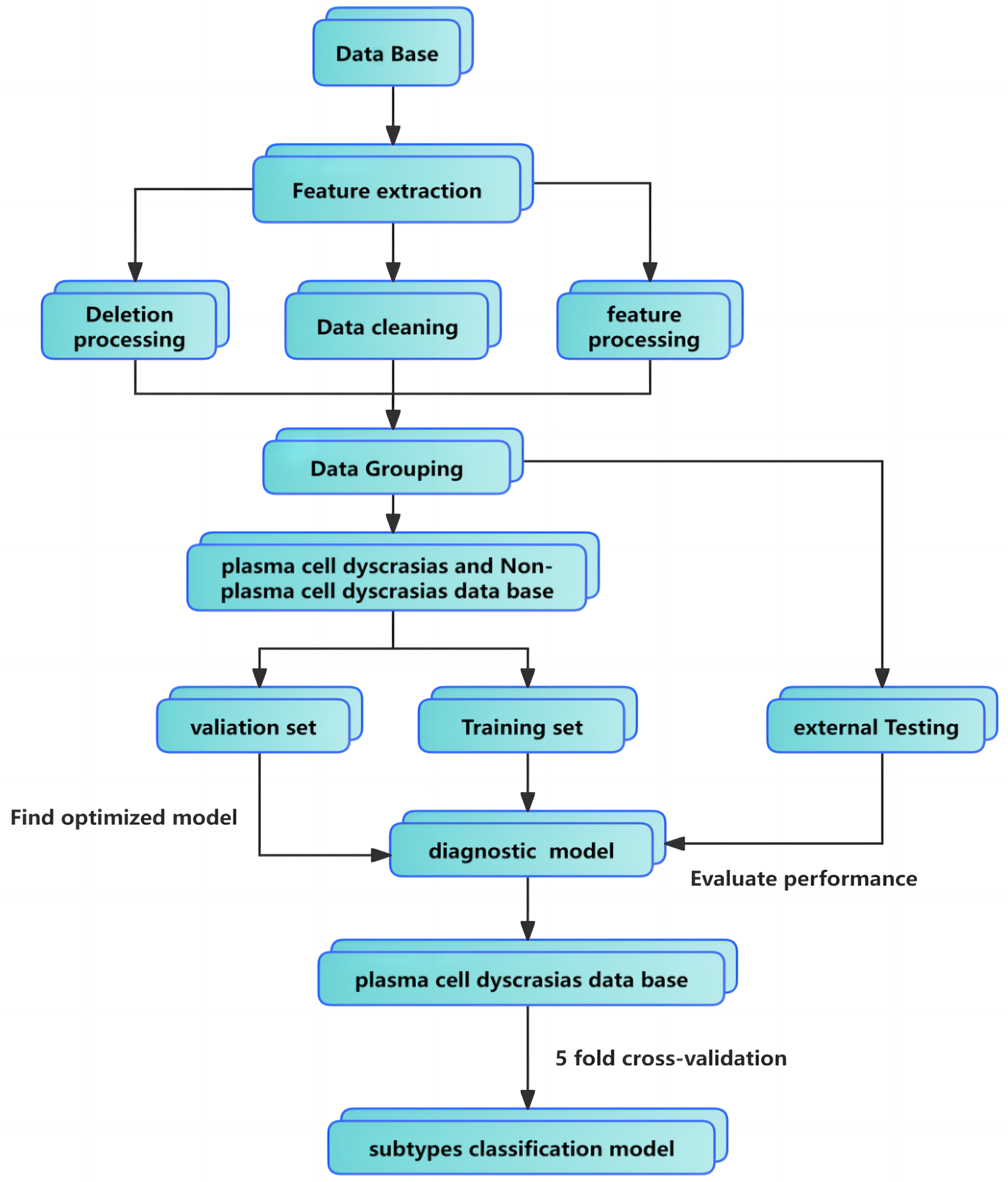
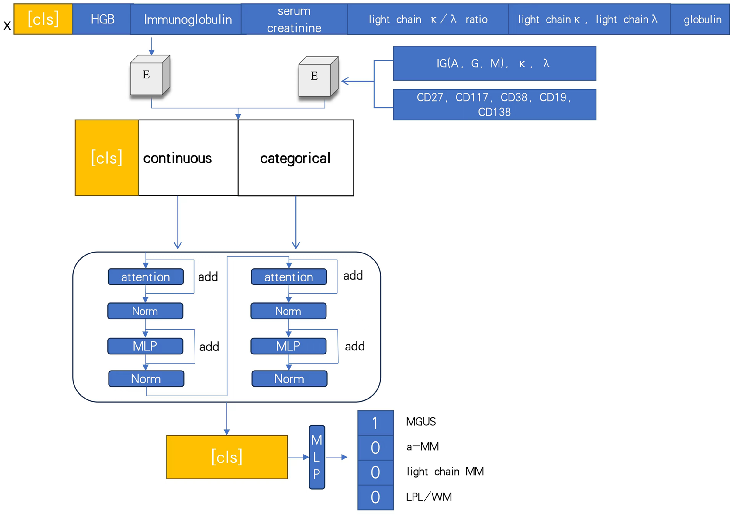
At diagnosis, bio-clinical parameters for each patient were assessed, including biomarkers associated with the CRAB criteria. The DNN model processed several indices, such as immunoglobulin, hemoglobin (HGB), serum creatinine, κ/λ light chain ratio, κ light chain, λ light chain, globulin, and immunofixation electrophoresis typing (IGA, G, M, κ, λ), along with CD markers (CD27, CD117, CD38, CD19, CD138). The mechanism-driven learning framework of the deep learning model is illustrated in Fig. 2.
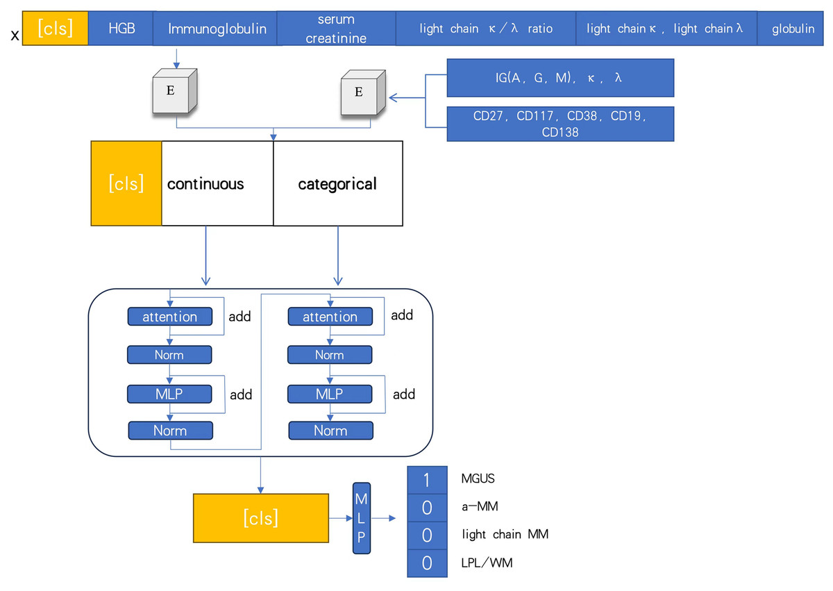
Figure 2: Deep neural networks model based on attention.
Improved loss function
In multi-class classification tasks, deep learning models commonly utilize the cross-entropy loss function to evaluate predictive performance. This function ensures that the model’s outputs remain within the range of 0 to 1. During optimization, gradient descent is employed to minimize the cross-entropy loss, guiding the model towards its optimal parameter configuration .
(4)
In predicting MM, the dataset contains a disproportionately higher number of MM cases. To enhance the model’s accuracy for rarer conditions, such as MGUS, a Logit adjustment was applied to the loss function (Menon et al., 2020). In this adjustment, represents the frequency of each class, denotes the model’s output, is a weighting factor, and ensures that the model’s output distribution more closely aligns with the true data distribution. As shown in the formula, Logit adjustment proportionally modifies the spatial distribution of based on the ratio of , thereby increasing the margin between and and assigning greater weight to underrepresented data.
(5)
Building on this foundation, the deep learning model was configured with a learning rate of 0.0001 and a batch size of 128. This setup ultimately enabled the successful classification and differentiation among a-MM, light chain MM, MGUS, and LPL within a dataset characterized by well-defined features.
Performance evaluation
1. Evaluation Indexes of a Diagnostic Model
Precision, recall, and F1 scores are standard metrics used to evaluate the performance of machine learning algorithms. These metrics are defined by the following equations.
(6)
(7)
(8)
Precision (P) measures the accuracy of correctly identifying plasma cell dyscrasias, while recall (R) reflects the proportion of true cases successfully detected. The F1 score balances precision and recall, with higher values indicating superior model performance. True positives (TP) represent correct classifications of plasma cell dyscrasias, false positives (FP) refer to instances mistakenly classified as dyscrasias, and false negatives (FN) are actual cases that were missed by the model. These metrics apply similarly to non-plasma cell dyscrasias.
2. Evaluation indexes of the subtype classification model
Performance evaluation utilized sensitivity (Se), specificity (Sp), positive predictive value (PPV), and negative predictive value (NPV), all calculated from the standard confusion matrix.
(9)
(10)
(11)
(12)
True positive, false positive, false negative, and true negative are represented as TP, FP, FN, and TN, respectively. In subtype classification models, these metrics are employed to evaluate various dimensions of model performance, offering insights into accuracy, precision, and effectiveness across different categories. By collectively considering these indices—sensitivity, specificity, PPV, and NPV—a comprehensive understanding of the model’s overall performance and suitability can be achieved. These metrics are essential for assessing the effectiveness of subtype classification models, providing valuable information on the model’s performance under different conditions.
All experiments referenced in this paper were conducted using Python version 3.10. The SVM and decision tree models were implemented through the scikit-learn library, while deep learning algorithms were developed using the PyTorch framework. The computational hardware used included an Intel i5-11400 CPU and an NVIDIA GeForce RTX 3060 GPU.
Results
1. Variable determination: To identify specific laboratory variables relevant to modeling plasma cell dyscrasias, a systematic comparison of 609 plasma cell dyscrasia patients and 579 control patients was performed. The distribution of clinical data is depicted in Fig. 3. Using a threshold of P < 0.05 in univariate and multivariate regression analyses, nine key variables were identified, as detailed in Tables 1 and 2. Demographic characteristics of the training, internal validation, and external validation sets, along with clinical features, are summarized in Table 3. According to the forest plot hazard ratio (Fig. 4), the nine variables selected for the diagnostic model included HGB, age, serum creatinine, ESR, κ/λ light chain ratio, κ light chain, λ light chain, globulin, and β2-microglobulin. The cluster heatmap (Fig. 5) and principal component analysis (PCA) (Fig. 6) demonstrated significant differences in the expression levels of these nine variables compared to the control group (liver, kidney, and rheumatic immune system diseases). Feature importance was ranked, and the final model was explained using the Shapley Additive Explanation (SHAP) method, as shown in Fig. 7.
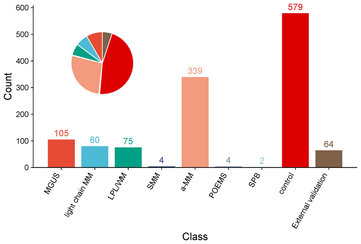
Figure 3: Pie chart and bar chart of proportions of a-MM, light chain MM, MGUS, LPL/WM, SMM, SPB, POEMS, control group and External validation in clinical data samples.
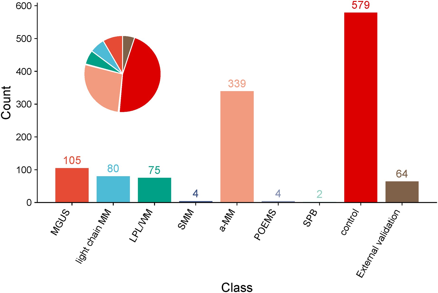
| Multivariate analysis | ||||
|---|---|---|---|---|
| Variables | HR | 95% CI, L | 95% CI, H | P-value |
| HGB (g/L) | 0.938 | 0.925 | 0.952 | 0.001 |
| Serum creatinine (μ mol/L) | 0.996 | 0.994 | 0.997 | 0.001 |
| ESR (mm/h) | 1.025 | 1.017 | 1.034 | 0.001 |
| Light chain κ/λ ratio | 1.235 | 1.136 | 1.342 | 0.001 |
| Light chain κ (g/L) | 1.004 | 1.002 | 1.006 | 0.001 |
| Light chain λ (g/L) | 1.004 | 1.002 | 1.006 | 0.001 |
| Albumin/globulin ratio | 2.631 | 0.996 | 6.951 | 0.051 |
| Albumin (g/L) | 0.984 | 0.937 | 1.033 | 0.512 |
| Globulin (g/L) | 1.033 | 1.014 | 1.052 | 0.001 |
| β2-microglobulin (mg/L) | 0.968 | 0.939 | 0.997 | 0.029 |
| Age (year) | 1.017 | 1.004 | 1.031 | 0.01 |
| Variables | Training (n = 950) |
Internal validation (n = 238) |
External validation (n = 64) |
|---|---|---|---|
| Sex (Male/Female) | 590/360 (62%/38%) | 140/98 (59%/41%) | 34/30 (53%/47%) |
| Age (years) | 65 (54, 74) | 66 (56, 75) | 63 (53, 72) |
| HGB (g/L) | 110 (88, 129) | 108.5 (89.75, 129.3) | 110 (87.75, 118.3) |
| Serum creatinine (μmol/L) | 93.10 (69.70, 151.80) | 90.50 (68.9, 138.9) | 91.90 (70.50, 151.3) |
| ESR (mm/h) | 26 (14, 50) | 30.00 (15.75, 58.00) | 15 (10, 39) |
| Light chain κ/λ ratio | 1.68 (0.71, 3.36) | 1.60 (0.54, 3.46) | 1.68 (1.14, 3.61) |
| Light chain κ (g/L) | 24.35 (10.43, 99.00) | 22.8 (10.0, 115.0) | 8.91 (6.60, 56.15) |
| Light chain λ (g/L) | 19.0 (5.6, 77.8) | 20.5 (6.5, 80.3) | 6.34 (4.35, 23.50) |
| Globulin (g/L) | 28.70 (24.00, 36.65) | 28.80 (23.40, 36.55) | 30.95 (22.15, 48.93) |
| β2-microglobulin (mg/L) | 3.1 (1.4, 6.5) | 3.5 (1.8, 5.8) | 4.45 (3.05, 7.58) |
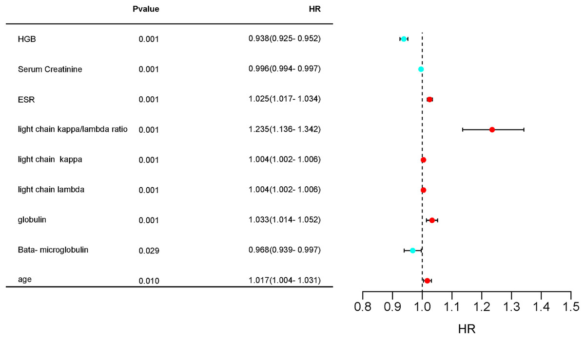
Figure 4: Forest plot hazard ratio of differential variables.
Hazard ratios (HR) and 95% confidence intervals (CI) and P-values for regression analysis in the “plasma cell dyscrasias” and “non-plasma cell dyscrasias” groups.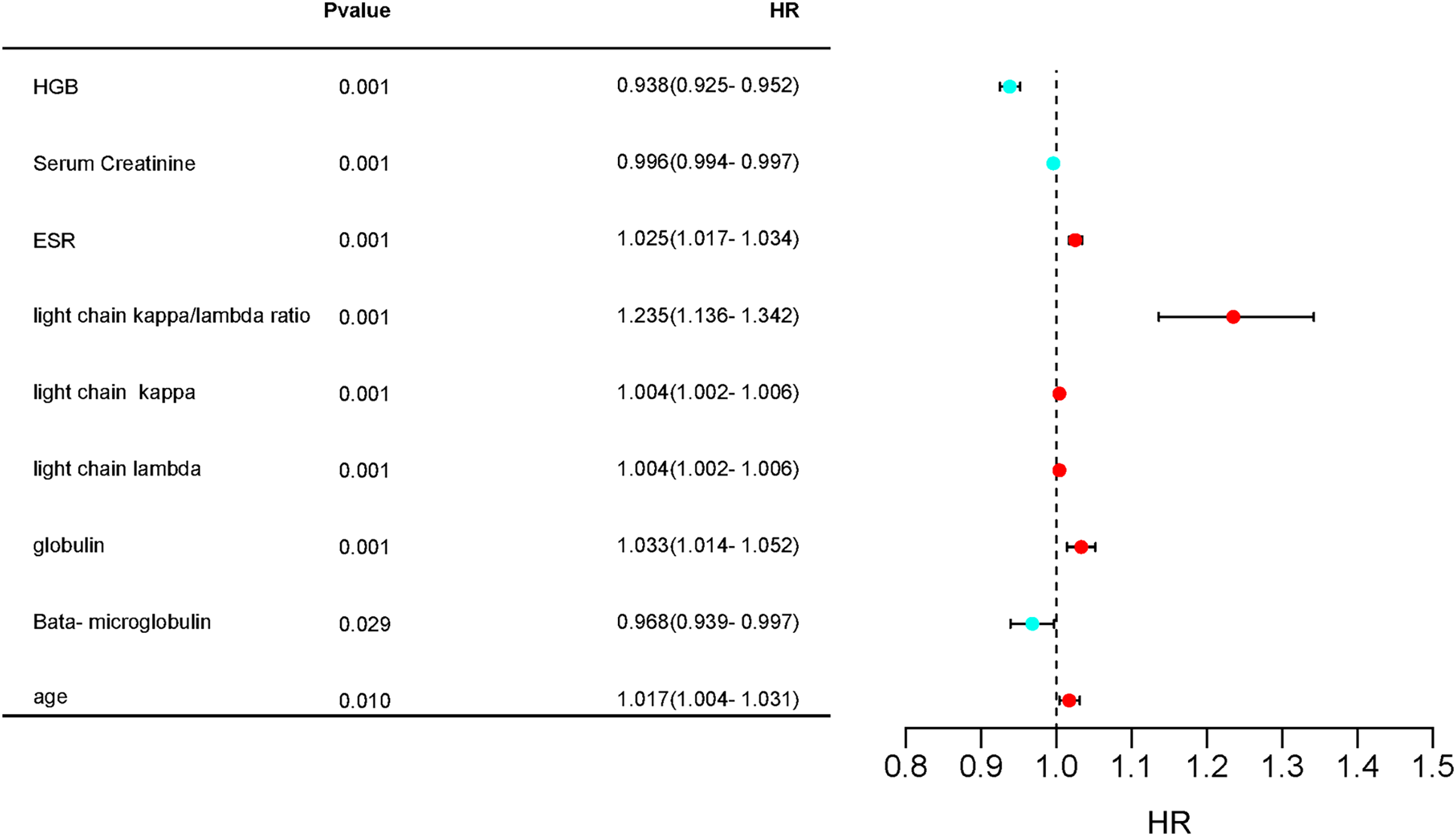
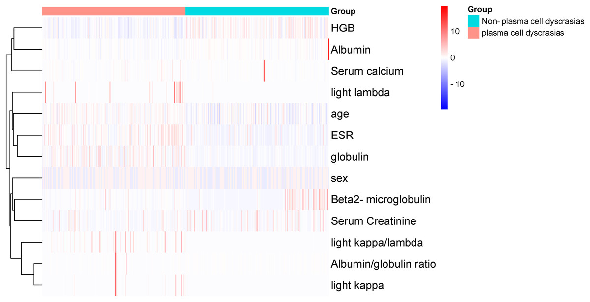
Figure 5: Cluster-heatmap in plasma and non-plasma cell dyscrasias using 13 laboratory variables paired with the heatmap package.
The color gradient reflects the difference in the variables between the two groups, namely HGB, age, serum creatinine, ESR, light chain κ/λ ratio, light chainκ, light chainλ, globulin, and ESR were the different variables.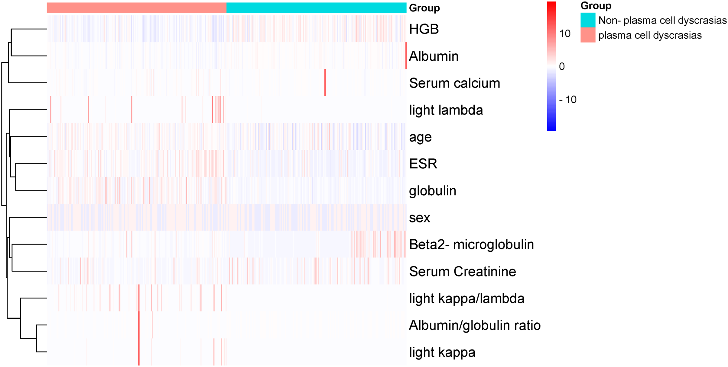
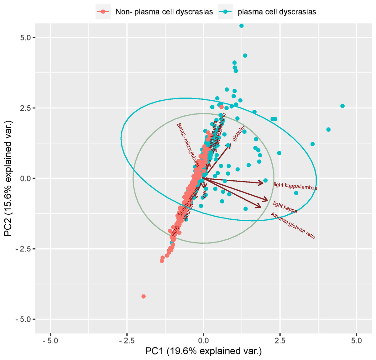
Figure 6: Principal component analysis (PCA).
Two-dimensional scatter plots represent sample distributions of the first two components obtained from principal component analysis (PCA) of 400 patients (randomly selected plasma cell dyscrasias n1 = 200, Non-plasma cell dyscrasias n2 = 200) based on evaluable data for the 13 characteristic parameters used for the analysis. Dots represent samples, and different colors represent different groups. The ellipse represents the core area of the grouping plus a default 68% confidence interval.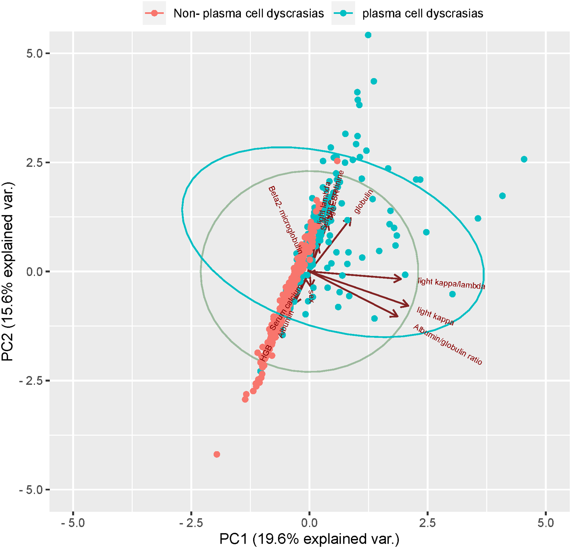
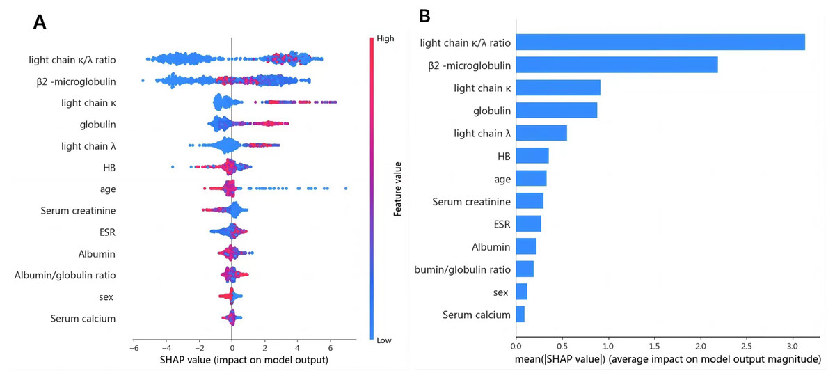
Figure 7: (A) SHAP summary dot plot; (B) SHAP summary bar plot.
The probability of plasma cell dyscrasia development increases with the SHAP value of a feature. A dot is made for the model’s SHAP value for each patient, so each patient has one dot on the line for each feature. The colors of the dots demonstrate the actual values of the features for each patient, as red means a higher feature value and blue means a lower feature value. The dots are stacked vertically to show density.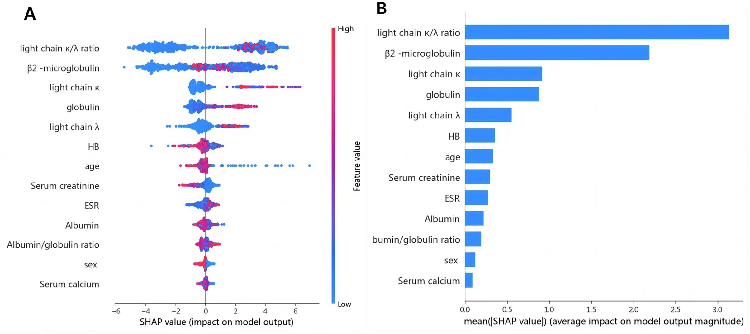
2. Diagnostic model performance: Several machine learning models, including SVM, DNN, decision tree, and GBDT, were trained and evaluated on the same dataset using the nine identified features: HGB, age, serum creatinine, ESR, κ/λ light chain ratio, κ light chain, λ light chain, globulin, and β2-microglobulin. Among these techniques, the GBDT model achieved a classification accuracy of 0.978 for non-myeloma dyscrasias and 0.935 for plasma cell dyscrasias. The GBDT model also achieved the highest recall rate (R) of 0.981 and the highest F1 score of 0.957 for plasma cell dyscrasias. Table 4 presents the P, R, and F1 scores for the four machine learning models.
| Method | Class | P | R | F1 |
|---|---|---|---|---|
| GBDT | Plasma cell dyscrasias | 0.935 | 0.981 | 0.957 |
| Non-plasma cell dyscrasias | 0.978 | 0.926 | 0.951 | |
| DNN | Plasma cell dyscrasias | 0.913 | 0.949 | 0.931 |
| Non-plasma cell dyscrasias | 0.947 | 0.908 | 0.927 | |
| Decision Tree | Plasma cell dyscrasias | 0.906 | 0.932 | 0.919 |
| Non-plasma cell dyscrasias | 0.923 | 0.894 | 0.908 | |
| SVM | Plasma cell dyscrasias | 0.858 | 0.883 | 0.871 |
| Non-plasma cell dyscrasias | 0.868 | 0.840 | 0.854 |
Additionally, the GBDT model recorded a false positive rate (FPR) of 1.93% and a false negative rate (FNR) of 4.17% for a-MM, supported by a specificity of 98.07% and sensitivity of 95.83%. These low FPR and FNR values emphasize the model’s robustness in differentiating plasma cell dyscrasias from other conditions, substantially minimizing the risk of misdiagnosis. By analyzing the receiver operating characteristic (ROC) curve, the area under the curve (AUC) was used to assess the classifier’s ability to distinguish between classes. A higher AUC indicates superior classification performance. Figure 8 shows the AUC performance of the four algorithms, with the GBDT classifier achieving an AUC of 0.987, outperforming the other models. The 95% confidence interval for the GBDT model was 0.984–0.993. AUC values for all four classifiers are illustrated in Fig. 8.
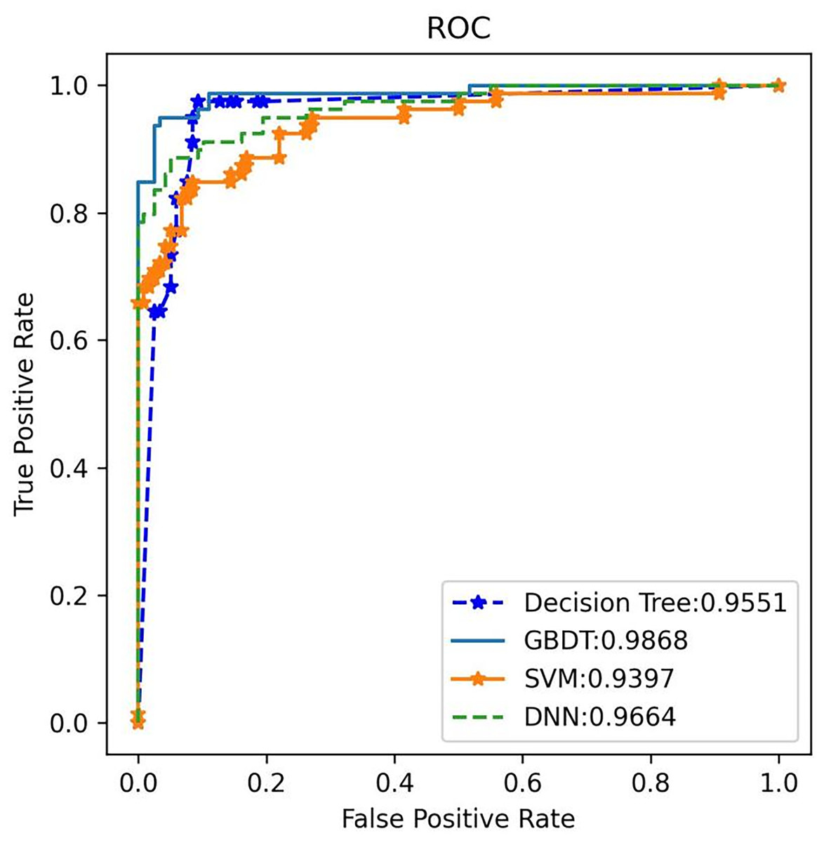
Figure 8: The ROC comparison of four algorithms based on nine variables (HGB, age, serum creatinine, ESR, light chain κ/λ ratio, light chainκ, light chainλ, globulin, β2 microglobulin).
The classifier with GBDT obtains an AUC of 0.987 (95% confidence interval (CI): [0.984–0.993]) and performs best when compared with the other three algorithms. ROC, Receiver Operating Characteristic; GBDT, Gradient Boosting Decision Tree; SVM support vector machine; DT, Decision Tree; DNN, Deep Neural Networks.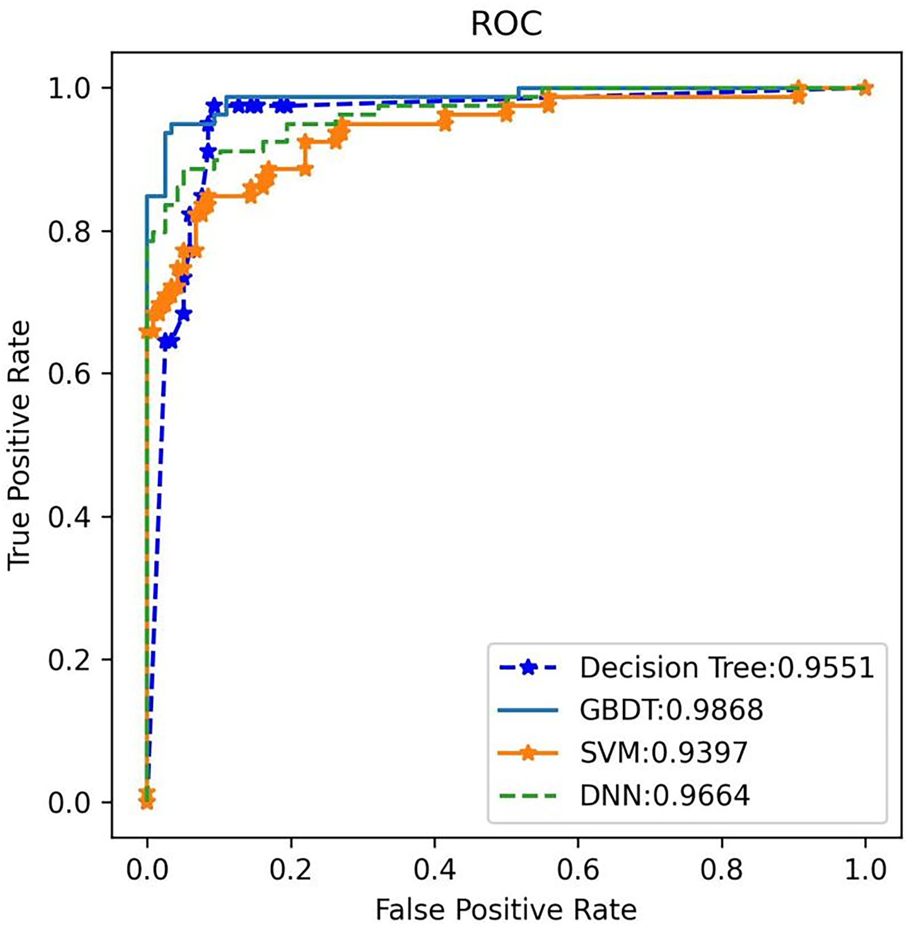
3. External validation: External validation was conducted using an independent test set to evaluate the performance of the four models. Once again, GBDT demonstrated the highest performance, achieving 100% accuracy, 97.1% recall, and an F1 score of 98.5% for plasma cell dyscrasias (as shown in Table 5). The GBDT classifier also recorded the highest AUC of 99%, as illustrated in Fig. 9. These results confirm that the selected GBDT model exhibits strong generalization and significant clinical utility.
| Method | Class | P | R | F1 |
|---|---|---|---|---|
| GBDT | Plasma cell dyscrasias | 1.000 | 0.971 | 0.985 |
| Non-plasma cell dyscrasias | 0.968 | 1.000 | 0.984 | |
| DNN | Plasma cell dyscrasias | 0.941 | 0.865 | 0.901 |
| Non-plasma cell dyscrasias | 0.833 | 0.926 | 0.877 | |
| Decision Tree | Plasma cell dyscrasias | 0.969 | 0.912 | 0.939 |
| Non-plasma cell dyscrasias | 0.906 | 0.967 | 0.935 | |
| SVM | Plasma cell dyscrasias | 0.762 | 0.941 | 0.842 |
| Non-plasma cell dyscrasias | 0.906 | 0.667 | 0.769 |
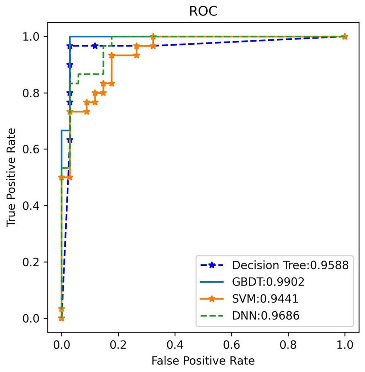
Figure 9: ROC Validation: ROC comparison of four algorithms based on nine variables for the external test set.
The external test classifier with GBDT has an AUC of 0.99 and performs best compared to the other three algorithms.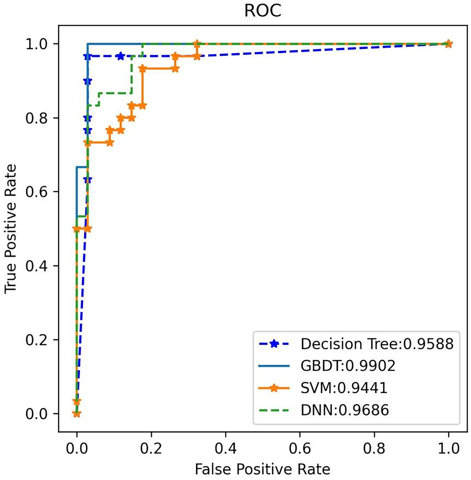
4. Subtype model results: For subtype classification of plasma cell dyscrasias, the DNN algorithm emerged as the optimal choice. The model’s performance in distinguishing between different plasma cell dyscrasia subtypes is summarized as follows:
MGUS: The model achieved an error rate (ER) of 9.52%, sensitivity of 90.48%, specificity of 96.36%, positive predictive value (PPV) of 90.48%, and negative predictive value (NPV) of 96.36%.
a-MM: The model showed an ER of 4.17%, sensitivity of 95.83%, specificity of 98.07%, PPV of 95.83%, and NPV of 98.07%.
Light chain MM: The DNN model achieved an ER of 6.25%, sensitivity of 93.75%, specificity of 98.33%, PPV of 93.75%, and NPV of 98.33%.
LPL: The model yielded an ER of 6.67%, sensitivity of 93.33%, specificity of 98.36%, PPV of 93.33%, and NPV of 98.36%. These results are detailed in Tables 6 and 7.
| Pathology | |||||
|---|---|---|---|---|---|
| Prediction | MGUS (n = 21) |
MM (n = 24) |
Light chain MM (n = 16) |
LPL/WM (n = 15) |
ER, % |
| MGUS, n | 19 | 1 | 1 | 0 | 9.52 |
| a-MM, n | 0 | 23 | 0 | 1 | 4.17 |
| Light chain MM, n | 1 | 0 | 15 | 0 | 6.25 |
| LPL/WM, n | 1 | 0 | 0 | 14 | 6.67 |
| Pathology | ||||
|---|---|---|---|---|
| Evaluation index | MAGUS | a-MM | Light chain MM | LPL/WM |
| Sensitivity, % | 90.48 | 95.83 | 93.75 | 93.33 |
| Specificity, % | 96.36 | 98.07 | 98.33 | 98.36 |
| Positive predictive value (PPV), % | 90.48 | 95.83 | 93.75 | 93.33 |
| Negative predictive value (NPV), % | 96.36 | 98.07 | 98.33 | 98.36 |
Discussion
Plasma cell disorders are a common type of hematologic malignancy, presenting significant diagnostic challenges due to the limited involvement of peripheral blood, making routine blood tests less effective for accurate diagnosis. Bone marrow morphology is widely regarded as the gold standard for diagnosing hematologic malignancies. However, as van de Donk et al. (2016) pointed out, in cases such as monoclonal gammopathy of undetermined significance (MGUS), bone marrow plasma cells may be absent, thus reducing the diagnostic accuracy of traditional morphological techniques. This highlights the need for more sensitive diagnostic tools capable of detecting early or occult diseases.
In recent years, AI has gained substantial attention in the medical field, with numerous studies demonstrating its potential in diagnosing hematologic malignancies. For instance, Clichet et al. (2022) developed a decision algorithm combining AI with multiparametric flow cytometry, achieving over 95% accuracy in distinguishing between plasma cell disorders such as MGUS, smoldering multiple myeloma (SMM), and MM. The AI algorithms used in this study, including GBDT and DNN, utilize advanced analytical methods to differentiate plasma cell disorders from similar conditions by examining specific hematologic and biochemical markers. Compared to traditional diagnostic methods, these AI models offer superior sensitivity and specificity, especially in scenarios with limited sample sizes or complex clinical presentations, where accuracy is significantly enhanced.
The lower false positive and false negative rates observed in this study further demonstrate the effectiveness of AI-based algorithms in diagnosing plasma cell disorders. Traditional diagnostic methods often struggle with sensitivity and specificity, particularly in early-stage or occult diseases. In contrast, the AI model used in this study showed notable improvements in both areas. Reducing false positives and negatives not only enhances diagnostic precision but also minimizes unnecessary follow-up testing and decreases the risk of delayed diagnosis. These findings underscore the significant potential of AI in clinical decision-making for hematologic malignancies.
A significant contribution of this study is the improved diagnostic performance achieved through the use of masking and continuous feature encoding techniques, which align with existing research on AI applications in high-dimensional biological data analysis (Jain & Xu, 2023). Furthermore, SHAP was employed for feature selection, identifying the most diagnostically relevant variables—a method validated in numerous clinical AI studies for its interpretability (Wang et al., 2024; Yi et al., 2023; Wang et al., 2022).
Despite these advancements, certain limitations persist. The data source and sample diversity were relatively limited, which may affect the model’s generalizability to broader populations. Additionally, further external validation is required to assess the long-term clinical utility of the model. As noted by Murphy et al. (2021) ethical and privacy concerns surrounding the use of AI in healthcare must also be addressed to ensure its responsible and sustainable integration into clinical practice (Witkowski, Okhai & Neely, 2024).
To overcome the constraints of a small external validation cohort and retrospective data, a prospective study with a larger and more diverse patient population is planned. This approach will enable the inclusion of additional diagnostic parameters, such as radiological data and advanced laboratory markers, strengthening the model’s robustness and generalizability. These future efforts will help ensure that the AI-based algorithm can be effectively applied across various clinical settings, improving both diagnostic accuracy and patient outcomes.
In conclusion, the findings highlight AI’s potential, particularly when combined with routine laboratory data, to significantly enhance early diagnostic capabilities for plasma cell disorders. Future work should prioritize model optimization, increased dataset diversity, and rigorous clinical validation to ensure long-term reliability and broad applicability.
Conclusion
This study utilized expected examination results from comprehensive hospital to train machine learning models, achieving automatic screening and precise classification of plasma cell disorders. Early alerts were generated through extensive data systems integrated with AI technologies. This approach holds significant potential for widespread application in comprehensive hospitals, enhancing the accuracy of plasma cell disorder classification while reducing the risk of missed diagnoses and misdiagnoses. Ultimately, an AI-driven early warning system for plasma cell abnormalities was successfully established.