
Molecular evidence that the Channel Islands populations of the orange-crowned warbler (Oreothlypis celata; Aves: Passeriformes: Parulidae) represent a distinct evolutionary lineage
- Published
- Accepted
- Received
- Academic Editor
- Michael Wink
- Subject Areas
- Biodiversity, Biogeography, Genetics, Taxonomy, Zoology
- Keywords
- Mitochondrial DNA, Microsatellites, Bird, Avian, Phylogeography, North America
- Copyright
- © 2019 Hanna et al.
- Licence
- This is an open access article distributed under the terms of the Creative Commons Attribution License, which permits unrestricted use, distribution, reproduction and adaptation in any medium and for any purpose provided that it is properly attributed. For attribution, the original author(s), title, publication source (PeerJ) and either DOI or URL of the article must be cited.
- Cite this article
- 2019. Molecular evidence that the Channel Islands populations of the orange-crowned warbler (Oreothlypis celata; Aves: Passeriformes: Parulidae) represent a distinct evolutionary lineage. PeerJ 7:e7388 https://doi.org/10.7717/peerj.7388
Abstract
We used molecular data to assess the degree of genetic divergence across the breeding range of the orange-crowned warbler (Oreothlypis celata) in western North America with particular focus on characterizing the divergence between O. celata populations on the mainland of southern California and on the Channel Islands. We obtained sequences of the mitochondrial gene ND2 and genotypes at ten microsatellite data for 192 O. celata from populations spanning all four recognized subspecies. We recovered shallow, but significant, levels of divergence among O. celata populations across the species range. Our results suggest that island isolation, subspecies (delineation by morphology, ecological, and life-history characteristics), and isolation-by-distance, in that order, are the variables that best explain the geographic structure detected across the range of O. celata. Populations on the Channel Islands were genetically divergent from those on the mainland. We found evidence for greater gene flow from the Channel Islands population to mainland southern California than from the mainland to the islands. We discuss these data in the context of differentiation in phenotypic and ecological characters.
Introduction
Oceanic islands have served as a natural laboratory for evolutionary studies for decades (Crawford, 2012). Patterns of phenotypic and genetic divergence on islands with varying degrees of isolation shed light on the processes of adaptation and speciation (Losos & Ricklefs, 2009; Greenberg & Danner, 2013) and provide data for evaluating traits that promote biodiversity (Lomolino, 2005; Gunderson, Mahler & Leal, 2018). Furthermore, comparisons of island taxa and their mainland counterparts are fundamental to assessing the taxonomic status of island endemics, many of which are of conservation concern (Wilson et al., 2009).
The California Channel Islands are well-known for their endemic or near endemic species and subspecies of birds (Johnson, 1972; Jones & Diamond, 1976). Of the forty-one native land bird species found on these islands, thirteen (32%) show phenotypic differentiation between the islands and mainland (Johnson, 1972). The islands are divided into two groups that differ geologically and biologically: the northern islands (San Miguel, Santa Rosa, Santa Cruz, and Anacapa) and the southern islands (San Nicolas, Santa Barbara, Santa Catalina, and San Clemente). Together, they extend for 260 km off the coast of southern California and range between 20 and 98 km from the mainland (Schoenherr, Feldmeth & Emerson, 1999). Patterns and processes of avian (especially passerine) diversification on the Channel Islands have been a topic of interest among ornithologists for decades (Diamond, 1969; Johnson, 1972; Lynch & Johnson, 1974; Greenberg & Danner, 2013). Apart from the following, few Channel Islands bird taxa have been the subject of published genetic studies: Aphelocoma californica and A. insularis (Delaney, Zafar & Wayne, 2008); Melospiza melodia (Wilson et al., 2009); Lanius ludovicianus, (Mundy, Winchell & Woodruff, 1997; Caballero & Ashley, 2011); Eremophila alpestris (Mason et al., 2014); and Artemisiospiza belli (Karin et al., 2018). Overall, these studies have shown that the Channel Islands harbor genetic distinctiveness in avian populations and that levels of divergence and gene flow between the islands and mainland vary among taxa.
The orange-crowned warbler (Oreothlypis celata) is currently divided into four subspecies that differ in plumage color (Figs. S1 and S2), size, molt patterns, habitat, song, and timing of migration and breeding (Foster, 1967; Dunn & Garrett, 1997; Gilbert, Sogge & Van Riper III, 2010). Oreothlypis celata celata (Say, 1823) breeds primarily in low, deciduous shrub-dominated thickets in northern North America, including most of Alaska through eastern Canada. Oreothlypis celata lutescens (Ridgway, 1872) prefers to nest in the dense riparian-chaparral ecotone with vertical structure provided by oaks or conifers along the Pacific coast from southeastern Alaska through California (Dunn & Garrett, 1997). Oreothlypis celata sordida (Townsend, 1890) nests in scrub and woodland on all eight California Channel Islands as well as on the Islas Coronado and Islas de Todos Santos off the northwestern coast of Baja California and in restricted areas on the coast of mainland southern California (Dunn & Garrett, 1997; Schoenherr, Feldmeth & Emerson, 1999). This subspecies is the only one that predominantly nests off the ground on the mainland (Gilbert, Sogge & Van Riper III, 2010). Oreothlypis celata orestera (Oberholser, 1905) nests in dense riparian areas and, at higher elevations, in stands of aspen groves in the Rocky Mountains from northern British Columbia through southern New Mexico and in some mountain ranges within the western deserts of North America (Dunn & Garrett, 1997).
Analyzing the geographic differentiation and distribution patterns of Channel Island birds, Johnson (1972) found evidence of both single and multiple colonization events, depending on the particular taxon. For Oreothlypis celata, he hypothesized that the insular O. c. sordida originated from a single colonization from the mainland to the northern Channel Islands, followed by differentiation and subsequent dispersal among the islands and recolonization of the mainland in areas that were locally unsuitable for O. c. lutescens. He also hypothesized that O. c. sordida is more closely related to Rocky Mountain O. c. orestera populations than to Pacific coast O. c. lutescens populations, suggesting a relictual pattern of evolution and distribution.
In the only published genetic study of Oreothlypis celata, Bull et al. (2010) used mitochondrial DNA (mtDNA) and microsatellite data to assess the relationships between northwestern North American populations of Oreothlypis celata celata and O. c. lutescens on Haida Gwaii, Canada. They found low, but statistically significant, differentiation between populations, suggesting recent divergence. They also found a pattern consistent with isolation-by-distance. However, because Bull et al. (2010) did not include the other two O. celata subspecies (O. c. orestera and O. c. sordida) in their analyses, their data do not provide insight into broader patterns and processes of differentiation across the species, including between Channel Islands and mainland populations.
In order to analyze broad-scale divergences among populations, we sampled mitochondrial and nuclear genetic data from all four subspecies of Oreothlypis celata. We assessed the relationship between Channel Island and mainland southern California populations and determined the relative rates of migration between these populations to test (Johnson, 1972) hypotheses about the origin and differentiation of O. celata on the Channel Islands. We discuss these data in the context of what is known about avian differentiation on the islands.
Materials and Methods
Population sampling
We obtained blood and/or frozen tissue samples from 192 Oreothlypis celata individuals collected between 1983 and 2009 (Table S1) from western North America representing each of the four subspecies (Table S1 and Fig. 1). To control for post-breeding dispersal, we used only samples collected during the breeding months of early April through July (Gilbert, Sogge & Van Riper III, 2010). We also obtained frozen tissue samples from two Nashville warblers (Oreothlypis ruficapilla) to use as outgroups in our analyses. We obtained samples from museum tissue collections (Table S1) and collected samples under California Department of Fish and Game scientific collecting permit numbers SC-458 and SC-10109, US Fish and Wildlife Service permit number MB153526, and with permission from the UC Berkeley Animal Care and Use Committee under Animal Use Protocols R285 and R317.
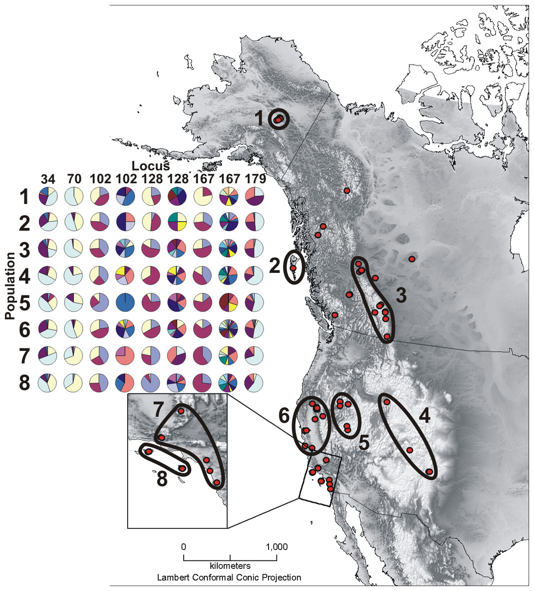
Figure 1: Sample map and microsatellite allele pie charts.
Depicted here are all Oreothlypis celata sampling localities and the associated population designations used in this study. Population numbers correspond to the “Pop #” column in Table 1. We also provide an across-population comparison of the percent prevalence of a subset of the alleles found in our samples for the three most variable (Vce102, Vce128, and Vce167) and three least variable (Vce34, Vce70, and Vce179) loci. For each population, we present the percent prevalence of both the three most common and the rare alleles. We define rare alleles as those whose average occurrence in populations represents less than 5% of the allele pool. Loci Vce70 and Vce102 were exceptions to this definition. Due to the small total number, we included all five detected alleles for Vce70. There were so many rare alleles for Vce102 that we defined the rare alleles for this locus as those with an average population occurrence of <1% of the total allele pool. For the least variable loci, we depict the percent prevalence of the three most common alleles and the rare alleles together in the same pie chart. Due to the large number of rare alleles in the most variable loci, we have depicted the rare alleles in a separate pie chart. For Vce102, Vce128, and Vce167, the left pie charts display the percent prevalence of the three most common alleles and the right graphs represent the percent prevalence of the rare alleles. The prevalence percentages depicted in the pie charts are all relative as the total prevalence of all alleles must sum to one. We recommend that the reader compare graphs vertically, across populations. A given color represents different alleles across columns.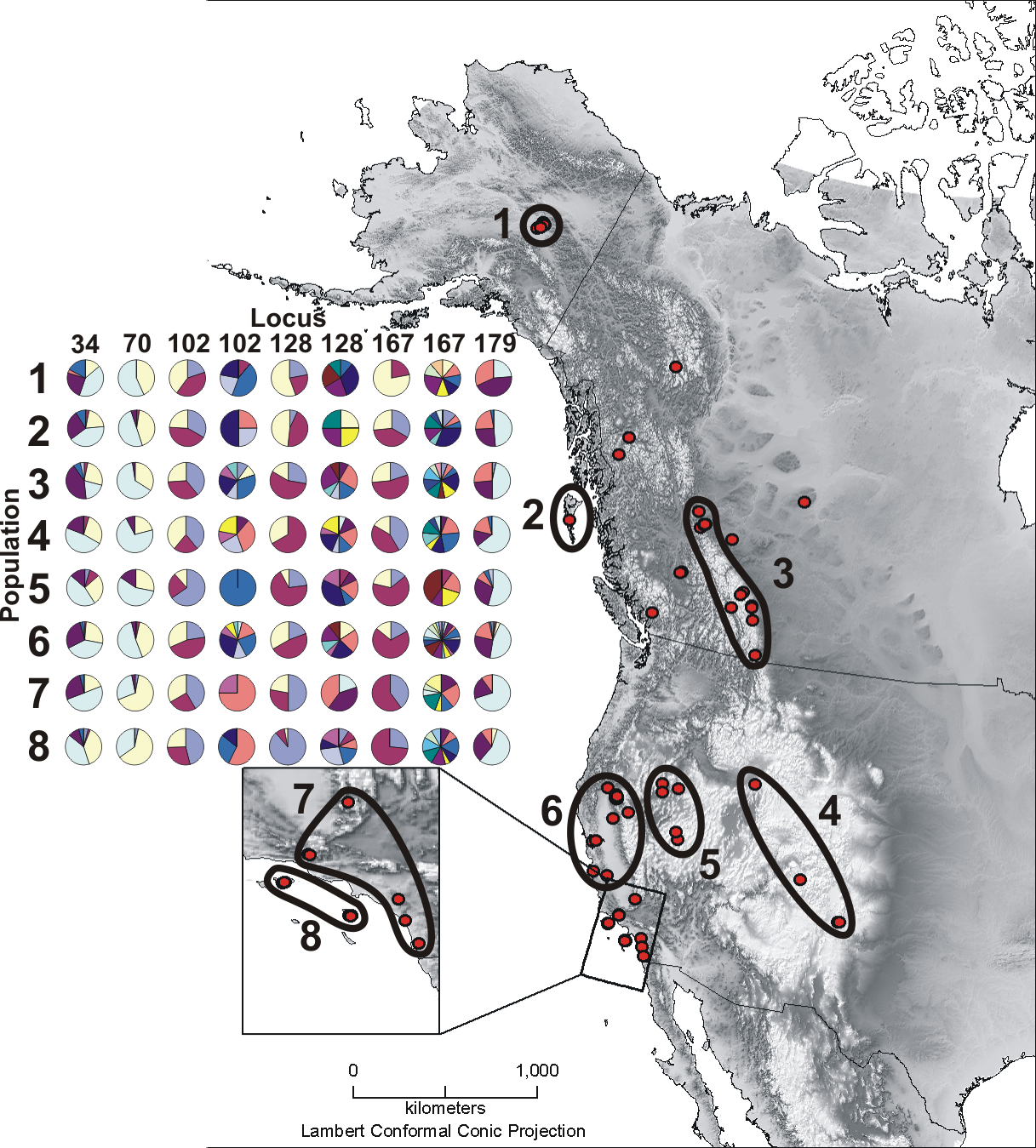
| Pop # | Population | N | Number of haplotypes | h | π | Tajima’s D | Fu’s Fs | Harpending’s Raggedness Index |
|---|---|---|---|---|---|---|---|---|
| North | 42 | 23 | 0.94+/-0.02 | 0.0029+/-0.0017 | −1.80* | −16.50** | 0.023 | |
| South | 92 | 42 | 0.94+/-0.01 | 0.0030+/-0.0017 | −2.35** | −26.42** | 0.018 | |
| 1 | Fairbanks | 15 | 9 | 0.89+/-0.06 | 0.0027+/-0.0017 | −1.16 | −3.05* | 0.126 |
| 2 | Haida Gwaii | 20 | 11 | 0.84+/-0.08 | 0.0028+/-0.0017 | −1.73* | −4.04* | 0.063 |
| 3 | Northern Rocky Mtns. | 19 | 11 | 0.89+/-0.06 | 0.0029+/-0.0018 | −1.31 | −4.19* | 0.030 |
| 4 | Southern Rocky Mtns. | 17 | 10 | 0.79+/-0.10 | 0.0019+/-0.0013 | −2.25** | −5.44** | 0.012 |
| 5 | Nevada | 16 | 10 | 0.83+/-0.10 | 0.0020+/-0.0013 | −2.10* | −5.51** | 0.041 |
| 6 | Northern California | 43 | 25 | 0.96+/-0.01 | 0.0037+/-0.0021 | −2.07* | −16.47** | 0.018 |
| 7 | Southern California | 16 | 9 | 0.85+/-0.08 | 0.0028+/-0.0017 | −1.71* | −2.66 | 0.105 |
| 8 | Channel Islands | 30 | 4 | 0.19+/-0.10 | 0.0002+/-0.0003 | −1.73* | −3.38** | 0.417 |
We examined populations at several hierarchical levels. First, we analyzed the data using all of the samples without a priori groupings. When these initial analyses revealed little spatial structure in the genetic data, we grouped the samples into eight populations (Fig. 1) based on their geographic proximity. This enabled us to explore the extent to which variation across ecosystem boundaries (geography) and present taxonomy (subspecies) are reflected in the genetic data. To explore the importance of geographic variation, we grouped the samples on either side of two separate geographic divisions: northern versus southern (populations 1–3 and 4–8, respectively, in Fig. 1) and coastal versus interior (populations 2, 6–8 and 1, 3–5, respectively, in Fig. 1). Our division between the northern and southern samples near the Pacific Coast fell at the southern limit of the Cascade Range in northern California. In the interior, we divided northern from southern samples between the Canadian Rocky Mountains and the Southern Rocky Mountains at the northern Idaho Clearwater River drainage. These landmarks are ecologically significant as they mark the southern extents of cedar-hemlock forest ecosystems (Brunsfeld et al., 2001) and have been hypothesized by many as sites of lineage contact in various taxa (Soltis et al., 1997; Swenson & Howard, 2005; Burg et al., 2006). We divided coastal from interior samples by designating as interior all areas east of the Alaska Range, Coast Mountains, the Cascades, and the Sierra Nevada, as splits between coastal and interior populations have been hypothesized in other warbler taxa (Bermingham et al., 1992). Finally, we grouped samples based on the four existing subspecific designations. We utilized each of these four separate sample groupings in subsequent analyses.
Laboratory procedures
We extracted DNA from blood or frozen tissues using a DNeasy Blood & Tissue Kit (Qiagen, Hilden, Germany) following the Qiagen protocol for animal tissues. We sequenced the mitochondrial genes NADH subunit 2 (ND2) and ATP Synthase subunit 6 (ATP6), both of which are commonly used in avian phylogeographic studies. We amplified a 1041 base pair (bp) fragment of the ND2 gene using the polymerase chain reaction (PCR) with primers L5204 and H6312 (Sorenson et al., 1999). PCR reactions (10 µL) contained 1X PCR Buffer (10 mm Tris-HCl, 1.5 mm M gCl2, 50 mm KCl, pH 8.3), 0.6 µm of each primer, 200 µm of each dNTP, 0.6 U of Taq and approximately 5–10 ng of genomic DNA. The PCR profile included an initial denaturation at 94 °C for 2 min; followed by 35 cycles of denaturation at 94 °C for 30 s, annealing at 53 °C for 30 s, and extension at 72 °C for 1 min; with a final extension at 72 °C for 10 min. We amplified a 704 bp fragment of the ATP6 gene by PCR using the primers a8PWL and C03HMH (Hunt, Bermingham & Ricklefs, 2001). The PCR profile followed that for the ND2 gene, except for annealing at 54 °C and extension for 45 s during the 35 cycle phase before the final extension.
We purified the PCR products using Exonuclease I and Shrimp Alkaline Phosphatase (ExoSAP-IT™; Applied Biosystems, Waltham, MA, USA) and sequenced the purified products using Big Dye terminator chemistry v. 3.1 (Applied Biosystems) and an AB PRISM 3730 DNA Analyzer (Applied Biosystems). We analyzed only samples for which we obtained sequences of both the forward and reverse DNA strands. We aligned complementary DNA strands, edited all sequences, detected stop codons, and aligned consensus sequences using Sequencher version 4.7 (Gene Codes Corporation, Ann Arbor, MI, USA). After obtaining 704 bp of ATP6 for 106 individuals, we detected the presence of a pseudogene in sequences and thus eliminated the ATP6 gene from further analyses.
We used ten polymorphic microsatellite markers (Vce34, Vce50, Vce70, Vce102, Vce103, Vce109, Vce116, Vce128, Vce167, and Vce179) developed for O. celata (Bowie et al., 2017). All ten loci were tetranucleotide repeats and three of them had imperfect core repeats. We amplified these microsatellites using PCR in 10 µL reactions containing: 1x PCR Buffer (10 mm Tris-HCl, 1.5 mm M gCl2, 50 mm KCl, pH 8.3), 0.6 µm of each primer, 200 µm of each dNTP, 0.6 U of Taq and approximately 5-10 ng of genomic DNA. The PCR conditions included one denaturation cycle at 94 °C for 2 min and 30 cycles consisting of 15 s of denaturation at 94 °C, 15 s of annealing at 50–55 °C, and 15 s of extension at 72 °C. We used T4 DNA polymerase (New England Biolabs, Ipswich, MA, USA) treatment to clean the PCR products of the Vce34, Vce50, Vce102, Vce103, Vce128, and Vce179 markers (Ginot et al., 1996). We mixed the samples with formamide and GS-500 LIZ size standard (Applied Biosystems) and analyzed them using an AB PRISM 3730 DNA Analyzer. We conducted allele binning and genotyping using Genemapper version 4.0 (Applied Biosystems).
Mitochondrial DNA analyses
We analyzed the ND2 sequences using maximum likelihood (ML), neighbor-joining (NJ), and maximum parsimony (MP) algorithms. We used RAxML BlackBox (Stamatakis, Hoover & Rougemont, 2008) to construct an ML tree with 100 bootstrap replicates and PAUP* version 4.0b10 (Swofford, 2003) to construct NJ and MP trees. Preliminary analyses of the mtDNA data using NJ, ML, and MP algorithms were not informative and intraspecific datasets often do not comply with the assumptions of MP and ML algorithms (Posada & Crandall, 2001). Therefore, we did not further explore tree-building methods that assume bifurcation of lineages by default and instead focused on the population genetics approaches described hereafter.
We generated a statistical parsimony network using TCS version 1.01 (Clement, Posada & Crandall, 2000) to visualize relationships among haplotypes and to analyze phylogeographic structure. In addition, we used analysis of molecular variance (AMOVA) in Arlequin version 3.1 (Excoffier, Smouse & Quattro, 1992; Excoffier, Laval & Schneider, 2007) to calculate the proportion of total mtDNA genetic variation explained by population groupings. The AMOVA provided estimates of overall FST and its analogue, ΦST (calculated using the Tamura-Nei model with a 0.05 gamma correction), using a non-parametric permutation approach to determine significance levels (Excoffier, Smouse & Quattro, 1992). We used Arlequin version 3.1 to examine genetic structure among population subdivisions by calculating pairwise FST and ΦST statistics (10,000 permutations) and applying sequential Bonferroni corrections when evaluating significance (Rice, 1989). We also used Arlequin version 3.1 to estimate haplotype diversity (h) and nucleotide diversity (π) (Nei, 1987), to calculate pairwise mismatch distributions for populations (Sum of Squared deviations and Harpending’s Raggedness index calculated to test goodness of fit; 10,000 bootstrap replicates), and to run two tests of selective neutrality, Tajima’s D (Tajima, 1989) and Fu’s F (Fu, 1997) tests.
We performed a spatial analysis of molecular variance (SAMOVA) using SAMOVA 1.0 (Dupanloup, Schneider & Excoffier, 2002) to assess the geographic arrangement of genetic structure. Unlike an AMOVA, this method does not require an a priori definition of populations. Instead, it uses sequence and geographic coordinate data (Lambert projection) to maximize the proportion of total genetic variation among populations (Dupanloup, Schneider & Excoffier, 2002). We identified the most likely partitioning of the samples by running SAMOVA 1.0 repeatedly with 2 to 20 groups and looking for the division assemblage with a maximized FCT (Dupanloup, Schneider & Excoffier, 2002).
Microsatellite analyses
We used Arlequin version 3.1 (Excoffier, Laval & Schneider, 2007) to calculate observed (HO) and expected (HE) heterozygosity values. We tested for Hardy–Weinberg equilibrium (HWE) and heterozygote deficiency using Genepop version 4.0.10 (10,000 dememorization steps, 1,000 batches, 10,000 iterations) (Raymond & Rousset, 1995; Rousset, 2008). In addition, we tested the microsatellite genotypes in each population and at each locus for linkage equilibrium using Genepop version 4.0.10 (10,000 dememorization steps, 1,000 batches, 10,000 iterations) (Raymond & Rousset, 1995), applying sequential Bonferroni corrections when evaluating significance (Rice, 1989). We examined null allele presence using Micro-Checker version 2.2.3 (Van Oosterhout et al., 2004) and used FSTAT version 2.9.3.2 (Goudet, 1995; Goudet, 2001) to estimate allelic richness (Rs), which controls for sample size when comparing the number of alleles among populations (Leberg, 2002).
We tested the proportion of total genetic variance explained by population groupings by performing an AMOVA (Excoffier, Smouse & Quattro, 1992) in Arlequin version 3.1, which provided estimates of overall FST. We calculated the significance levels for the AMOVA using a non-parametric permutation approach (10,000 permutations) (Excoffier, Smouse & Quattro, 1992). We examined genetic structure among population subdivisions by calculating pairwise FST values using Arlequin version 3.1 (10,000 permutations) and pairwise RST values using RSTCALC version 2.2 (Goodman, 1997), applying sequential Bonferroni corrections for multiple simultaneous comparisons when evaluating significance (Rice, 1989).
We tested the pairwise correlation between direct geographic and genetic (Nei, 1972) distances (isolation-by-distance) among all individuals sampled by conducting a Mantel test using GenAlEx version 6.1 (Peakall & Smouse, 2006; Peakall & Smouse, 2012). We also used GenAlEx version 6.1 to run a principal coordinates analysis (PCA) in order to examine the organization of the genetic structure.
In a further effort to detect spatial organization in our sample assemblage, we analyzed our dataset of ten microsatellite loci using Structure version 2.3.4 (Pritchard, Stephens & Donnelly, 2000; Falush, Stephens & Pritchard, 2003; Hubisz et al., 2009; Pritchard, Falush & Hubisz, 2012). This method uses Bayesian clustering to examine genetic frequencies across loci and attempts to identify the number of clusters (K) based on the likelihood values for varying K values. We performed preliminary analyses without providing any information concerning population designations. After these initial analyses, we then designated eight populations in the input and used this information as a prior (LOCPRIOR) (Hubisz et al., 2009) in further analyses to improve population discrimination. We implemented the analyses using the admixture model with correlated allele frequencies (Falush, Stephens & Pritchard, 2003), examined K = 1 − 20, executed a 100,000 MCMC iteration burn-in, and then performed 1,000,000 subsequent MCMC iterations. We replicated the simulation at each K twenty times. To assist in identifying the optimal K, we used Structure Harvester version 0.6.94 (Earl & VonHoldt, 2012; Earl, 2014), which uses the Evanno, Regnaut & Goudet (2005) method to identify the number of clusters. We ran Structure and Structure Harvester using StrAuto version 1.0 (Chhatre & Emerson, 2017; Chhatre & Emerson, 2018) with GNU Parallel version 20141022 (Tange, 2011). To align clusters across the Structure runs, we ran CLUMPP version 1.1.2 (Jakobsson & Rosenberg, 2007) and then used a modified version of Distruct version 2.2 (Raj, Stephens & Pritchard, 2014; Chhatre, 2016; Hanna, Cicero & Bowie, 2018) to plot the clusters.
Based on the results of the Structure analysis described above, we ran two additional Structure analyses to check for the presence of substructure. We first analyzed the Channel Islands samples with the samples from Santa Cruz Island and Santa Catalina Island split into separate populations. We used the parameters as detailed above, including the LOCPRIOR for K = 1 − 10. We then analyzed the seven remaining populations with the same parameters as above for K = 1 − 20.
In order to assess the relative rate of migration between the Channel Islands and mainland southern California, we ran IMa2p version 58a0260 (Sethuraman & Hey, 2015; Sethuraman, 2017). We input both the ND2 sequences and microsatellite genotypes and performed three separate runs each with 15 chains, 1,000,000 burnin steps, and 2,000,000 further steps following the burnin. We have provided further methodology details in ocwa-popgen version 1.0.0 on GitHub (Hanna, Cicero & Bowie, 2018).
Results
mtDNA sequence variation
We obtained a complete 1041 bp fragment of the mtDNA ND2 gene for 192 Oreothlypis celata and two O. ruficapilla individuals; there were no missing data and no insertions, deletions, or gaps. After merging identical sequences, we found 72 unique haplotypes (Table S1 ) with 81 variable sites. We found no evidence for selection (P = 0.702) between Oreothlypis celata sequences and two sequences of the closely related O. ruficapilla (Lovette, Bermingham & Sheldon, 2002).
mtDNA haplotype network
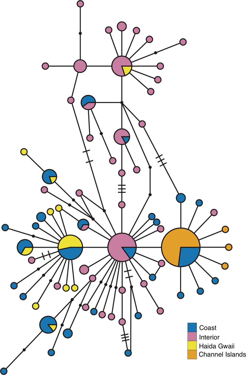
Examination of the statistical parsimony network revealed shared alleles, regardless of how we grouped samples into populations (Fig. 2 and Fig. S3). The haplotypes clustered largely along a north-south geographic axis, but the majority of the Haida Gwaii Oreothlypis celata possessed haplotypes in the “southern” group. Three mutational differences separate the major haplotype clusters of the northern and southern O. celata with some outlier individuals falling into each grouping.
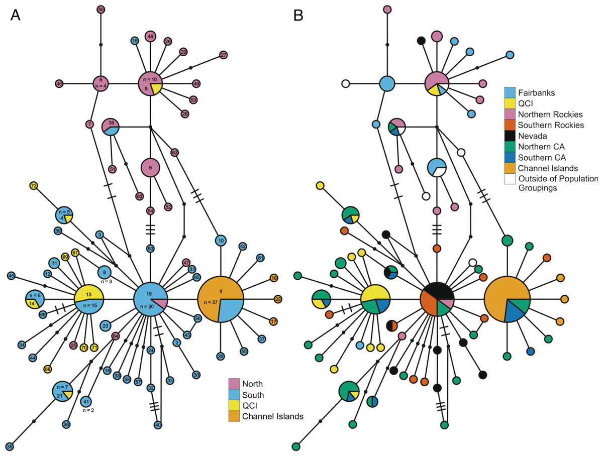
Figure 2: ND2 haplotype network.
(A) depicts the ND2 haplotype network shaded according to samples’ designation in the northern or southern population. (B) is the haplotype network shaded using sample assignment under the eight population grouping arrangement, a more fine-scale partitioning than the north-south grouping schema. The haplotype numbers in (A) correspond with the numbers in Table S1. Circle sizes are proportional to the number of individuals with each haplotype. Lines connect haplotypes that differ by one mutation. Dots represent inferred haplotypes. Hash marks indicate the number of mutations between haplotypes separated by more than one mutational difference. For one circle of each size, we have labeled the number of individuals represented by that circle following “n =”.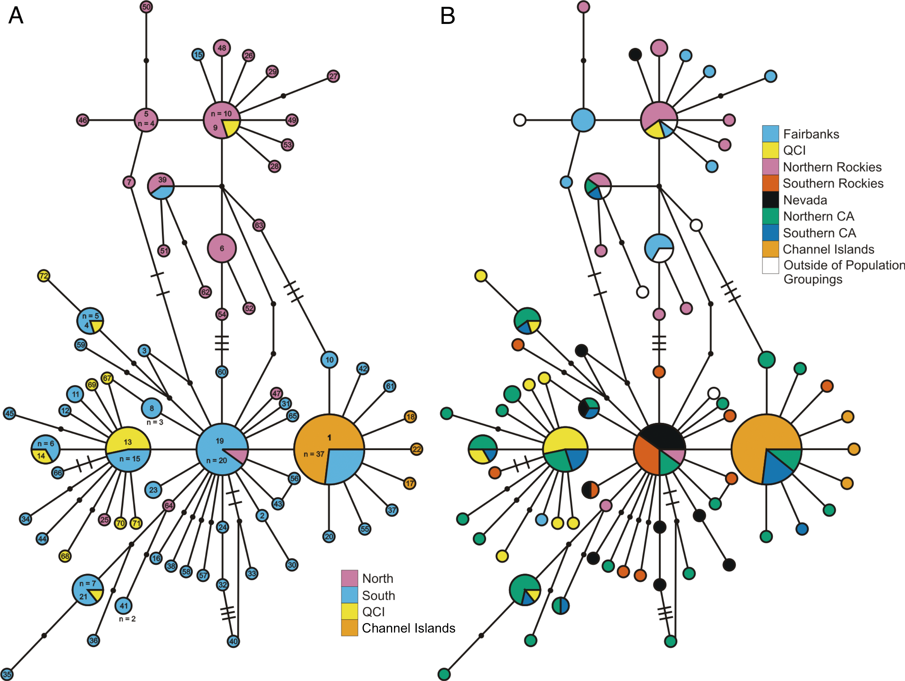
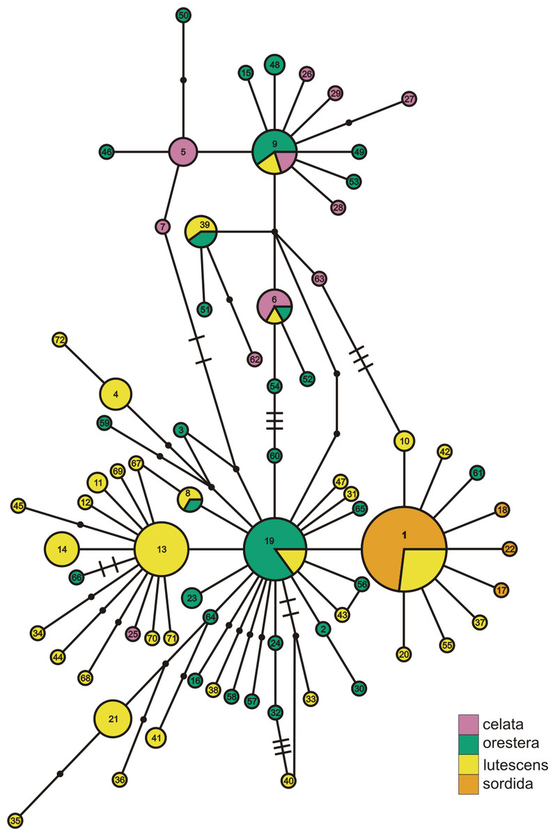
Figure 3: ND2 haplotype network with subspecies population grouping.
This is the ND2 haplotype network colored by the subspecies designations of samples. The haplotype numbers correspond with the numbers in Table S1. The size of each circle is proportional to the number of individuals with that haplotype. Lines connect haplotypes that differ by one mutation. Dots represent inferred haplotypes. Hash marks indicate the number of mutations between haplotypes separated by more than one mutation.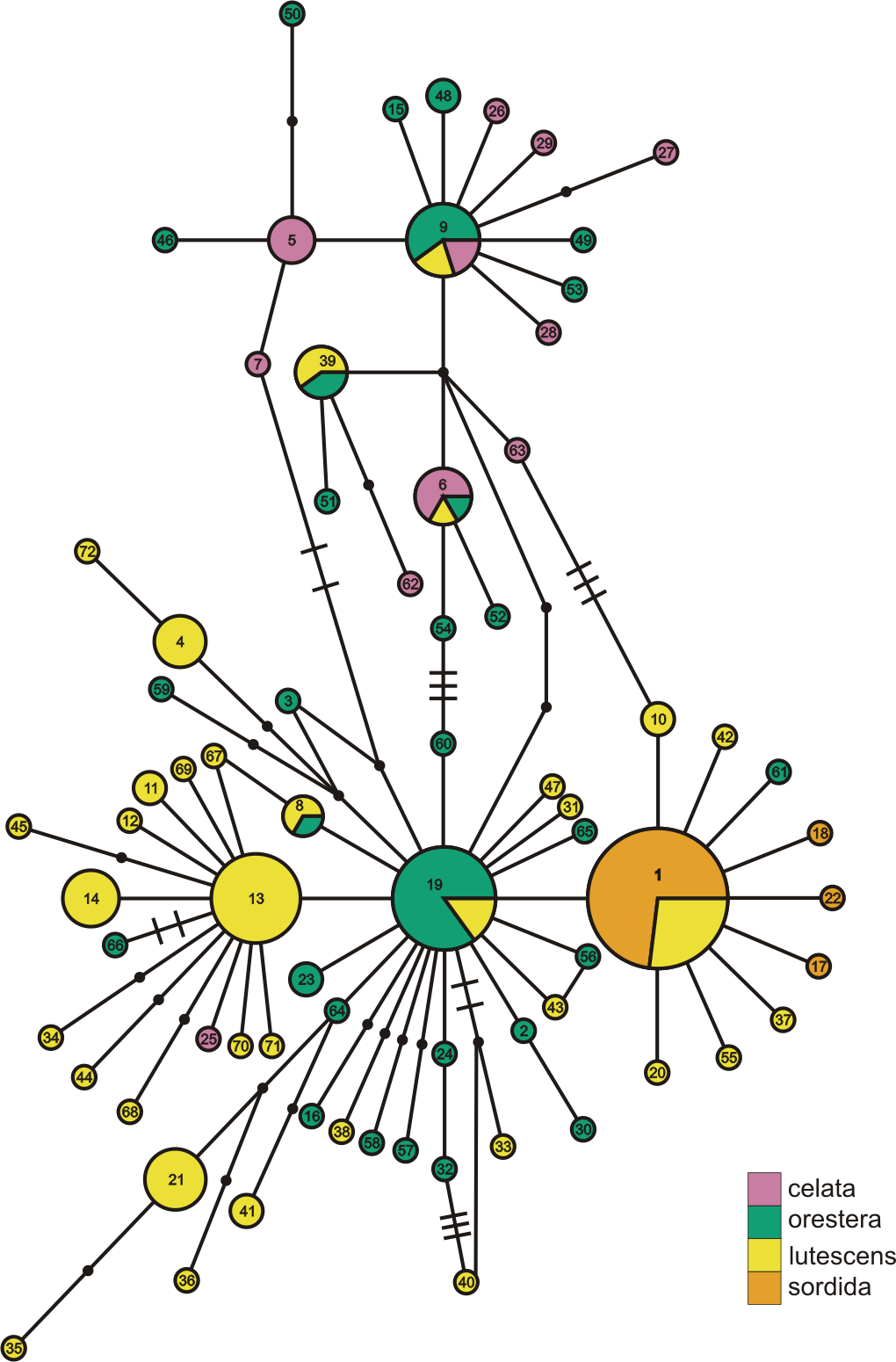
The Oreothlypis celata haplotypes from the Channel Islands clustered much more tightly than those from Haida Gwaii. We found four ND2 haplotypes among the Channel Islands O. c. sordida, but the majority of individuals shared a single haplotype; the three other Channel Islands haplotypes appeared only in one individual each (Fig. 2). There was at most one mutational difference between the haplotype of a Channel Islands O. celata and the next Channel Islands haplotype. Although we found three singleton, private Channel Islands ND2 haplotypes, individuals from northern and southern California shared the most common Channel Islands haplotype. The Haida Gwaii samples, with eleven haplotypes, were more loosely clustered than the Channel Islands samples with a maximum of nine mutational steps between individuals (Fig. S3).
When we identified samples by subspecies (Fig. 3), we found no interior Oreothlypis celata orestera individuals that shared haplotypes with the Channel Islands O. c. sordida. We did, however, find O. c. orestera haplotypes that were one mutational step away from O. c. sordida haplotypes (Fig. 3). The main cluster of O. c. lutescens haplotype diversity was separated from the O. c. sordida haplotype cluster by a haplotype more often found in O. c. orestera than in O. c. lutescens. The haplotypes did not appear to cluster across a coast-interior axis (Fig. S3). However, with the exception of one Haida Gwaii haplotype, the island populations of the Channel Islands and Haida Gwaii did not share haplotypes with any individuals from interior populations.
Population structure inferred from mtDNA
Variability in mtDNA sequences differed among populations (Table 1). We found that the Channel Islands population had the lowest nucleotide diversity (0.2 × 10⁻³) of all eight populations, whereas the northern California population had the highest (3.7 × 10⁻³). The nucleotide diversity of the Haida Gwaii population (2.8 × 10⁻³) was substantially higher than that of the Channel Islands populations and equaled that of the southern California population (2.8 × 10⁻³). When grouped into northern and southern population clusters, the two groupings contained almost exactly the same nucleotide diversities (2.9 × 10⁻³ and 3.0 × 10⁻³, respectively).
Although the statistical parsimony networks (Figs. 2, 3 and S3) did not display evidence of reciprocal monophyly among populations or subspecies, the AMOVA revealed significant differentiation in haplotype frequencies for each of the four alternative groupings of our samples. Overall FST estimates from our AMOVA analysis of ND2 sequences were all highly significant (p < 0.01) for samples grouped into: (1) northern and southern clusters (0.191); (2) eight populations (0.202); (3) coastal and interior clusters (0.186); and (4) subspecies (0.195). Overall ΦST estimates were greater than the FST estimates for the different population data sets, and were also all highly significant with p < 0.01: (1) northern-southern (0.429); (2) eight-population (0.365); (3) coastal-interior (0.254); and (4) subspecies (0.299). The pairwise population FST values reflected patterns that were nearly congruent to the pairwise ΦST estimates, so we have chosen to present only the pairwise ΦST estimates (Tables 2–4).
| Fairbanks | Haida Gwaii | Northern Rocky Mountains | Southern Rocky Mountains | Nevada | Northern California | Southern California | Channel Islands | |
|---|---|---|---|---|---|---|---|---|
| Fairbanks | – | 0.525* | 0.011 | 0.584* | 0.532* | 0.486* | 0.528* | 0.809* |
| Haida Gwaii | 0.029 | – | 0.481* | 0.152* | 0.166* | 0.061 | 0.110 | 0.564* |
| Northern Rocky Mountains | 0.005 | 0.002 | – | 0.521* | 0.467* | 0.440* | 0.472* | 0.754* |
| Southern Rocky Mountains | 0.119* | 0.087* | 0.026 | – | 0.006 | 0.016 | 0.047 | 0.531* |
| Nevada | 0.141* | 0.092* | 0.033 | 0.000 | – | 0.035 | 0.069 | 0.558* |
| Northern California | 0.027 | 0.020 | 0.000 | 0.038* | 0.054* | – | 0.000 | 0.245* |
| Southern California | 0.103* | 0.079* | 0.025 | 0.089* | 0.095* | 0.040 | – | 0.261* |
| Channel Islands | 0.221* | 0.177* | 0.094* | 0.145* | 0.123* | 0.111* | 0.027 | – |
| North | South | Haida Gwaii | Channel Islands | |
|---|---|---|---|---|
| North | – | 0.479* | 0.492* | 0.681* |
| South | 0.011 | – | 0.094* | 0.228* |
| Haida Gwaii | 0.013 | 0.038* | – | 0.564* |
| Channel Islands | 0.130* | 0.091* | 0.178* | – |
| Lutescens | Orestera | Celata | Sordida | |
|---|---|---|---|---|
| lutescens | – | 0.126* | 0.469* | 0.232* |
| orestera | 0.021* | – | 0.258* | 0.375* |
| celata | 0.016 | 0.046* | – | 0.786* |
| sordida | 0.106* | 0.105* | 0.187* | – |
Pairwise population FST and ΦST estimates (0.036 and 0.000, respectively) between Santa Cruz Island (northern Channel Islands) and Santa Catalina Island (southern Channel Islands) were not significant. However, pairwise ΦST estimates supported the collective Channel Islands as a distinct population. Pairwise ΦST values between the Channel Islands and every other population were significant, ranging from 0.245 to 0.809 with the samples grouped into eight populations (Table 2) and from 0.228 to 0.681 with the samples grouped into northern and southern clusters (Table 3). With the samples grouped into eight populations, we estimated the highest pairwise ΦST values between the Channel Islands and the two northern, interior populations (Fairbanks, 0.809; Northern Rocky Mountains, 0.754). Of all of the pairwise comparisons involving the Channel Islands, we estimated the lowest ΦST between the Channel Islands and the northern and southern California populations (0.245 and 0.261, respectively).
Pairwise ΦST estimates between Haida Gwaii and every other population within the set of eight populations were significant, except for those between Haida Gwaii and the northern and southern California populations. Of all of the Haida Gwaii pairwise comparisons, pairwise ΦST was highest (0.564) between the Haida Gwaii and Channel Islands populations. The pairwise ΦST estimate was significant between the northern and southern populations (0.479; Table 3), but it was not as high as the estimate between the northern and Haida Gwaii populations (0.492). In contrast, pairwise ΦST was much lower between Haida Gwaii and the southern population (0.094; Table 3).
With the samples grouped by subspecies (Table 4), we estimated significant pairwise ΦST between Oreothlypis c. sordida and all other subspecies, with the lowest values between O. c. sordida and O. c. lutescens (0.232) and the highest between O. c. sordida and O. c. celata (0.786). Oreothlypis c. lutescens and O. c. orestera had the lowest pairwise ΦST value of all of the subspecies comparisons. All of the pairwise ΦST estimates were significant when we grouped the samples by subspecies (Table 4) and by coastal versus interior populations (Table S2).
SAMOVA
As we found with our maximum parsimony and maximum likelihood analyses, our SAMOVA analyses indicated that deep genetic structure is not present in our mitochondrial sequence data set. We never obtained a maximized FCT with the SAMOVA analyses, so we could not reject panmixia or obtain support for population structure greater than K = 1. SAMOVA is known to perform poorly in the presence of isolation-by-distance (Dupanloup, Schneider & Excoffier, 2002) and we recovered significant isolation-by-distance in the microsatellite data. However, the trend was weak and likely did not greatly affect the SAMOVA analyses. Although we never recovered a maximized FCT with the SAMOVA analyses, we examined the groupings created for K = 2 − 4 to see whether the analyses recovered any divisions between northern, southern, and island samples. These analyses partitioned the samples in general agreement with our northern and southern sample groupings. For K = 2, we recovered one group composed entirely of northern samples. The second group included all of the southern, Channel Islands, and Haida Gwaii samples as well as samples from five coastal and interior localities (in British Columbia, Alberta, and Fairbanks) in our designated northern population. Grouping samples with K = 3 and K = 4 created partitions within the northern and southern populations but were not consistent with subspecies boundaries.
Mismatch distributions
Mismatch profiles that follow a Poisson distribution suggest population growth following an event such as a range expansion (Rogers & Harpending, 1992; Harpending et al., 1993). Multimodal mismatch profiles can suggest a number of different population dynamic scenarios, such as constant size (Slatkin & Hudson, 1991; Rogers & Harpending, 1992; Harpending et al., 1998), expanding fronts (Liebers, Helbig & De Knijff, 2001), and geographic structuring resulting from restricted gene flow (Marjoram & Donnelly, 1994). All populations had negative Tajima and Fu statistics and all were statistically significant with the exception of the Fairbanks and Northern Rocky Mountains populations for Tajima’s D and the southern California population for Fu’s F (Table 1). Harpending’s Raggedness indices were not statistically significant for mismatch distributions in any of the populations, indicating that we could not reject a population expansion hypothesis (Table 1). The northern, southern, and Channel Islands populations displayed mismatch profiles following a Poisson distribution, suggesting recent population growth (Fig. 4). With the samples grouped into eight populations, we observed mismatch profiles with a Poisson distribution in all populations except the Fairbanks and Haida Gwaii populations, both of which appeared to have multimodal mismatch profiles (Fig. 4).
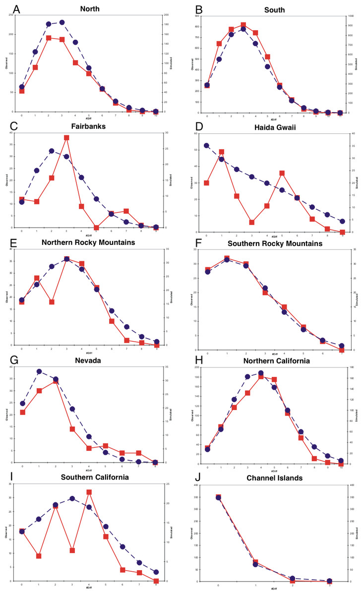
Figure 4: Mismatch distributions.
(A–J) are mismatch distributions for ten populations. Square points connected by smooth lines represent observed distributions. Circular points connected by dotted lines represent expected distributions for a growing population with the same mean.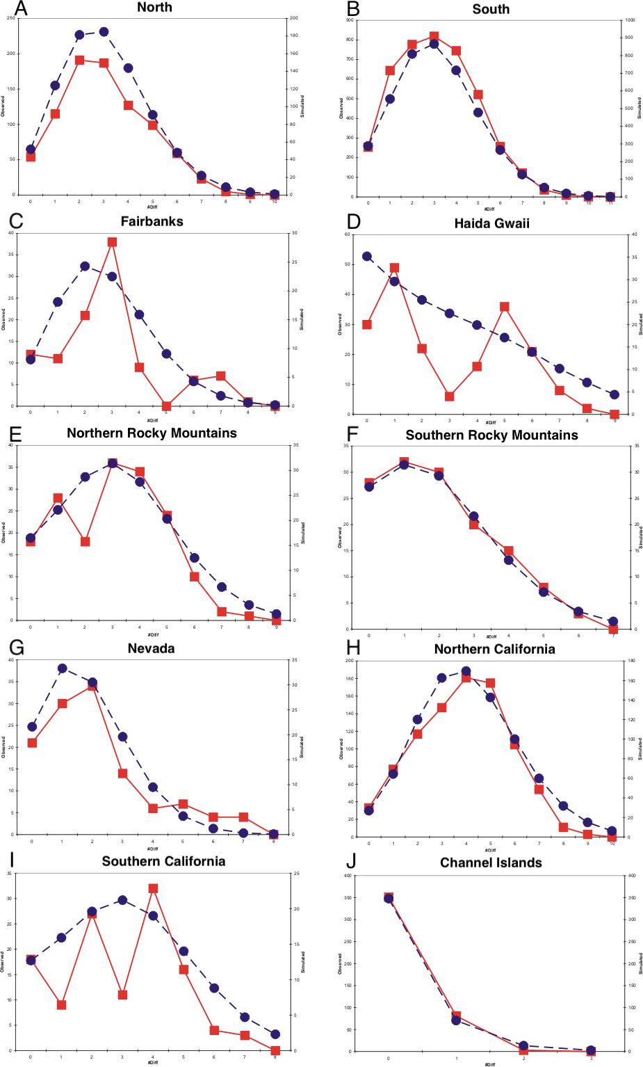
Population structure inferred from microsatellite data
We successfully obtained genotypes for 192 Oreothlypis celata individuals at ten microsatellite loci with no missing data apart from three individuals for which we were unable to genotype a subset of the loci (Table 5, Figs. S3 and S4). We found no evidence for null alleles in any microsatellite locus in any population. In addition, there was no evidence for linkage disequilibrium in the northern, southern, Channel Islands, or Haida Gwaii populations; no disequilibrium tests were significant after we applied Bonferroni corrections. We did not observe deviation of observed heterozygosity from Hardy-Weinberg equilibrium (HWE) expectations repeatedly across loci in any of the populations resulting from our various methods of sample grouping. Observed heterozygosity at all ten loci did not differ from that expected under HWE for the northern, southern, Channel Island, and Haida Gwaii population set. However, locus Vce34 was out of HWE in the Fairbanks population, locus Vce167 was out of HWE in the interior population, and locus Vce34 was out of HWE in the O. c. celata population.
The overall FST estimates from our analysis of microsatellite genotypes for the northern-southern, eight-population, coastal-interior, and subspecies population sets (0.017, 0.022, 0.016, 0.020, respectively) were all highly significant (p < 0.001). Overall RST estimates were also highly significant (p < 0.001), exhibiting the same pattern as the FST estimates and exceeded these for the northern-southern, eight-population, coastal-interior, and subspecies population sets (0.055, 0.068, 0.053, 0.058, respectively).
Both the pairwise FST and RST estimates from our microsatellite data displayed patterns almost congruent to the pairwise FST and ΦST estimates obtained from the mtDNA data. As with the pairwise FST and ΦST estimates for the mtDNA data, the pairwise population FST values were smaller than and showed patterns similar to the pairwise RST estimates, so we chose to present only pairwise RST estimates (Tables 2–4, and Table S3) here. As with the pairwise ΦST estimates, the pairwise RST estimates supported the existence of a distinct Channel Islands population. In further agreement with the mtDNA analyses, the pairwise FST and RST estimates between Santa Cruz Island and Santa Catalina Island (representing the northern and southern Channel Islands, respectively) were not statistically significant. Pairwise RST estimates between the Channel Islands population and the northern, southern, and Haida Gwaii populations were significant at 0.130, 0.091, and 0.178, respectively (Table 3). When we grouped samples into eight populations, pairwise RST values between the Channel Islands and every other population, except for southern California, were significant, ranging from 0.027 to 0.221 (Table 2). Within the set of eight populations, the highest pairwise RST estimate (0.221) was between the Channel Islands and Fairbanks populations. Of the pairwise comparisons amongst the set of eight populations that included the Channel Islands, the lowest pairwise RST estimate (0.027) was between the Channel Islands and southern California populations; the second-lowest estimate (0.094) was between the Channel Islands and Northern Rocky Mountains. Across all loci, we identified three private alleles in the Channel Islands and four in Haida Gwaii, whereas we found only two private alleles in the southern California population (Table S3). When we grouped samples by subspecies, the highest of the pairwise RST estimates involving O. c. sordida (0.187) was between O. c. sordida and O. c. celata. The lowest of these estimates (0.105) was between O. c. sordida and O. c. orestera, but the estimate between O. c. sordida and O. c. lutescens (0.106) was very close (Table 2).
| Population | Locus | N | A (Private Alleles) | RS | HO | HE | p-val |
|---|---|---|---|---|---|---|---|
| North | |||||||
| Vce34 | 43 | 10 (1) | 8.51 | 0.698 | 0.827 | 0.085 | |
| Vce50 | 43 | 37 (4) | 24.14 | 0.953 | 0.966 | 0.738 | |
| Vce70 | 42 | 4 (0) | 3.66 | 0.452 | 0.555 | 0.177 | |
| Vce102 | 42 | 12 (3) | 9.664 | 0.738 | 0.836 | 0.223 | |
| Vce103 | 42 | 8 (0) | 7.011 | 0.571 | 0.640 | 0.059 | |
| Vce109 | 42 | 10 (1) | 8.331 | 0.833 | 0.833 | 0.381 | |
| Vce116 | 42 | 10 (2) | 8.146 | 0.786 | 0.839 | 0.331 | |
| Vce128 | 42 | 18 (0) | 14.43 | 0.857 | 0.924 | 0.211 | |
| Vce167 | 43 | 23 (4) | 17.00 | 0.814 | 0.915 | 0.097 | |
| Vce179 | 43 | 8 (0) | 6.869 | 0.860 | 0.788 | 0.190 | |
| South | |||||||
| Vce34 | 94 | 10 (0) | 7.428 | 0.798 | 0.804 | 0.633 | |
| Vce50 | 93 | 42 (7) | 21.90 | 0.946 | 0.962 | 0.029 | |
| Vce70 | 94 | 5 (0) | 3.711 | 0.500 | 0.571 | 0.643 | |
| Vce102 | 94 | 13 (3) | 9.119 | 0.766 | 0.827 | 0.250 | |
| Vce103 | 94 | 12 (3) | 6.884 | 0.574 | 0.634 | 0.067 | |
| Vce109 | 94 | 14 (3) | 8.691 | 0.840 | 0.810 | 0.070 | |
| Vce116 | 94 | 10 (1) | 7.471 | 0.830 | 0.813 | 0.829 | |
| Vce128 | 94 | 20 (0) | 13.31 | 0.883 | 0.892 | 0.141 | |
| Vce167 | 94 | 28 (6) | 17.08 | 0.872 | 0.914 | 0.569 | |
| Vce179 | 94 | 11 (2) | 7.593 | 0.840 | 0.779 | 0.424 | |
| Haida Gwaii | |||||||
| Vce34 | 20 | 7 (0) | 7.000 | 0.650 | 0.797 | 0.277 | |
| Vce50 | 20 | 24 (3) | 24.00 | 1.000 | 0.962 | 1.000 | |
| Vce70 | 20 | 4 (0) | 4.000 | 0.550 | 0.581 | 0.141 | |
| Vce102 | 20 | 7 (0) | 7.000 | 0.550 | 0.772 | 0.064 | |
| Vce103 | 20 | 8 (0) | 8.000 | 0.650 | 0.669 | 0.899 | |
| Vce109 | 20 | 9 (0) | 9.000 | 0.700 | 0.853 | 0.029 | |
| Vce116 | 20 | 7 (1) | 7.000 | 0.900 | 0.792 | 0.224 | |
| Vce128 | 20 | 9 (0) | 9.000 | 0.750 | 0.768 | 0.493 | |
| Vce167 | 20 | 16 (0) | 16.00 | 0.900 | 0.935 | 0.813 | |
| Vce179 | 20 | 7 (0) | 7.000 | 0.650 | 0.740 | 0.271 | |
| Channel Islands | |||||||
| Vce34 | 30 | 9 (0) | 8.308 | 0.700 | 0.779 | 0.364 | |
| Vce50 | 30 | 23 (2) | 19.18 | 0.900 | 0.945 | 0.562 | |
| Vce70 | 30 | 3 (0) | 2.893 | 0.500 | 0.505 | 0.725 | |
| Vce102 | 30 | 7 (0) | 6.549 | 0.800 | 0.802 | 0.375 | |
| Vce103 | 30 | 2 (0) | 2.000 | 0.467 | 0.364 | 0.295 | |
| Vce109 | 30 | 8 (0) | 7.678 | 0.833 | 0.829 | 0.650 | |
| Vce116 | 30 | 8 (0) | 7.409 | 0.700 | 0.789 | 0.144 | |
| Vce128 | 29 | 14 (1) | 11.85 | 0.724 | 0.704 | 0.467 | |
| Vce167 | 29 | 15 (0) | 13.82 | 0.655 | 0.902 | 0.006 | |
| Vce179 | 30 | 7 (0) | 6.549 | 0.833 | 0.775 | 0.820 |
When we grouped samples into northern, southern, Channel Islands, and Haida Gwaii populations, we found that the pairwise RST estimates between Haida Gwaii and the southern population were significant, but we did not find significance between Haida Gwaii and the northern population nor between the northern and southern populations. When we grouped the samples into eight populations, the pairwise RST estimates involving the Haida Gwaii population ranged from 0.002 with the Northern Rocky Mountains to 0.177 with the Channel Islands; estimates were significant with all populations, except for Fairbanks, the Northern Rocky Mountains, and northern California (Table 2). The pairwise RST estimates did not suggest much differentiation within the northern populations, as none of the pairwise RST estimates involving the Fairbanks, Haida Gwaii, Northern Rocky Mountains, and northern California populations were statistically significant (Table 2). The insignificant pairwise RST estimate between the Southern Rocky Mountains and Nevada suggested a connection between these populations; pairwise RST estimates between them and all other populations, except for the Northern Rocky Mountains, were significant (Table 2).
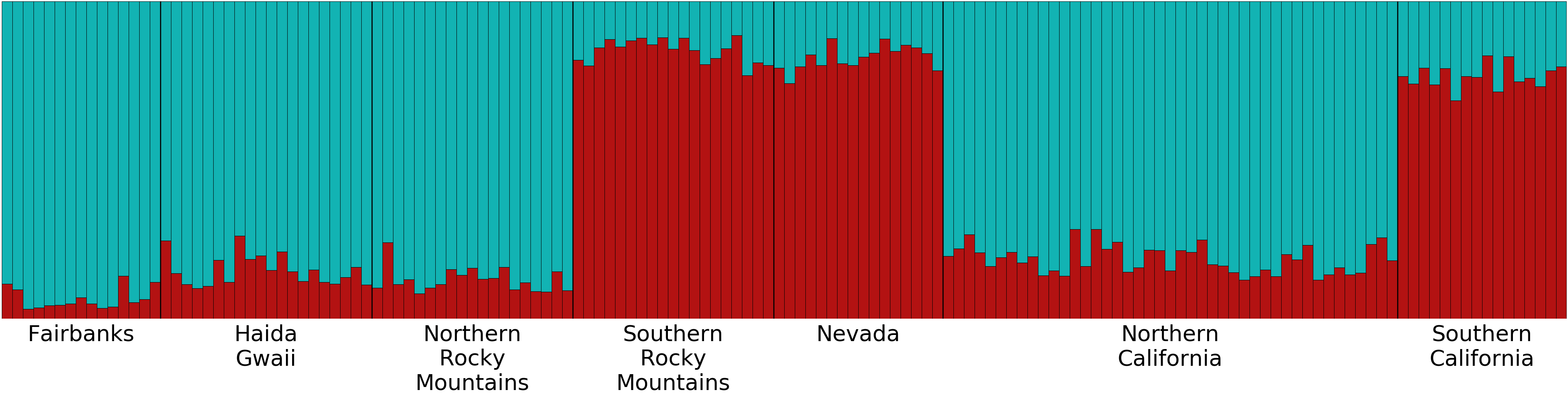
Overall, the microsatellite data revealed little genetic structure and low divergence of populations among our Oreothlypis celata samples. Our PCA analysis did not reveal distinct clustering of the samples by population. Mantel tests utilizing geographic distance (GGD) and Log(1+GGD) versus genetic distance (GD) resulted in weak, statistically significant, positive correlation between geographical distance of O. celata sampling localities and genetic distance measured at microsatellite loci (r2 = 0.015, P = 0.006 for GGD vs. GD and r2=0.031, P = 0.001 for Log(1+GGD) vs. GD). Our preliminary Structure analyses, in which we did not provide any a priori population information, suggested K = 1 as the optimal number of genetic clusters. When we grouped the samples into eight pre-designated populations, the mean ln Pr(X—K) and ΔK (Evanno, Regnaut & Goudet, 2005) suggested K = 2 as the optimal number of genetic clusters (Fig. 5). All of the Channel Islands samples had high ancestry (>83%) in one of the clusters, whereas the northernmost samples had the highest ancestry in the other cluster. In our analysis of substructure within the seven populations other than the Channel Islands, ΔK suggested K = 2 as optimal, but the highest mean ln Pr(X — K) was for K = 1, although the log probability for K = 2 was very similar. With K = 2, the southern California, Nevada, and Southern Rocky Mountains populations had high ancestry in one of the clusters and the northern California, Northern Rocky Mountains, Haida Gwaii, and Fairbanks populations had similarly high ancestry in the other genetic cluster (Fig. S4). In our analysis of substructure within the Channel Islands samples, ΔK suggested K = 4 as optimal, but the highest mean ln Pr(X — K) was for K = 1.
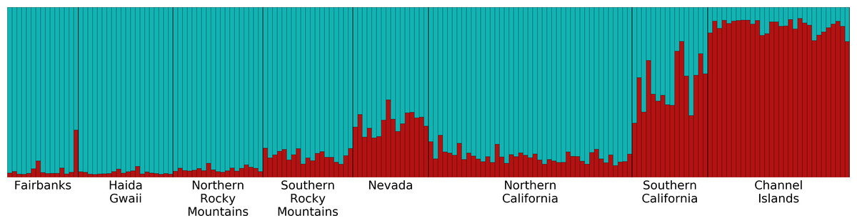
Figure 5: Structure plot for K = 2 with Channel Islands population included.
Different colors represent the two genetic clusters identified by Structure. Each vertical bar represents an individual Oreothlypis celata. The height of each color in a given bar illustrates the proportion of ancestry derived from each genetic cluster for that individual. When sample locality was excluded as a prior, we recovered K = 1.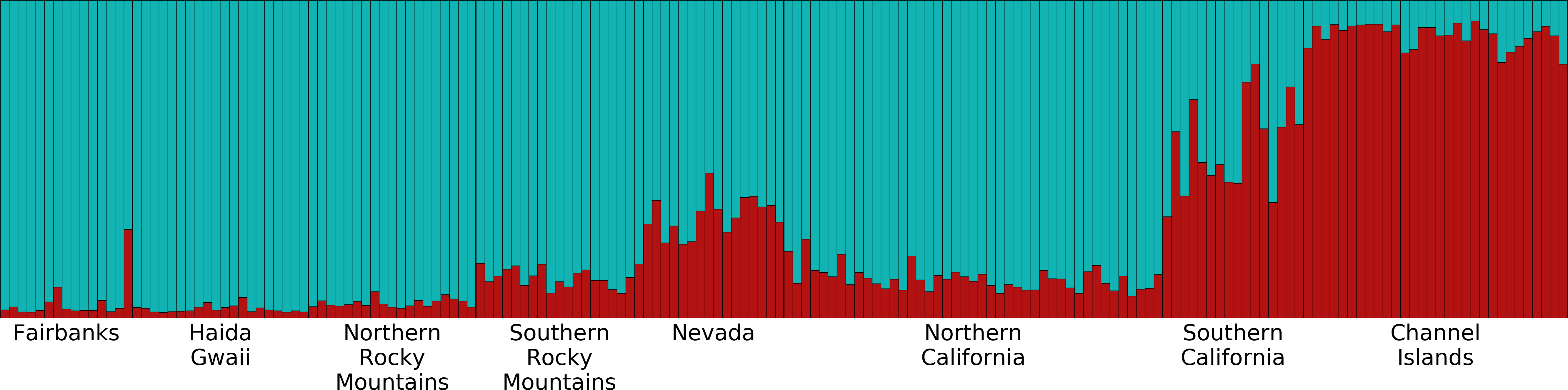
Migration rate estimates
Our IMa2p analyses obtained an upper bound to the effective size of the Channel Islands population, but the analyses did not converge on an upper bound to the effective size of the mainland southern California population. This suggests that the effective size of the mainland population is likely much higher than that of the Channel Islands. Even though we were unable to accurately calculate migration rates scaled by population size, we were still able to assess the relative population sizes and rates of migration between the two populations. Across all three runs, we calculated a pairwise probability of 1.000 that the current effective population size of the southern California population is greater than that of the Channel Islands population. The probability that the current effective population size of the Channel Islands population is greater than that of the southern California population was <0.001. Our migration rate estimates were similar across our three IMa2p runs. Across all three runs, we estimated probabilities of 0.986 to 1.000 that the rate at which (looking forward in time) the southern California population receives genes from the Channel Islands population is greater than that of the reverse direction. Inversely, we calculated probabilities ranging from 0.000–0.013 that the rate at which (looking forward in time) the Channel Islands receives genes from southern California is greater than migration in the reverse direction.
Discussion
Genetic analyses of population structure in Oreothlypis celata revealed some structure in portions of the range and high levels of shared alleles across much of the mainland distribution of O. celata. The strongest result derived from our present dataset is that both the mitochondrial and microsatellite data suggested that the Channel Islands represent the most genetically distinct population included in our study. We found the highest genetic divergence between the Channel Islands and Fairbanks populations, the two most geographically distant populations in our analyses. More generally, the mitochondrial data suggested higher pairwise divergences among populations than the microsatellite data. The mitochondrial, but not the microsatellite data, supported statistically significant divergence between northern and southern O. celata. The microsatellite data provided weak support for isolation-by-distance across the species range.
Both the mtDNA and microsatellite data suggested that the Channel Islands Oreothlypis celata comprise a separate population that is distinct from the mainland population. Notable is the lack of ND2 haplotype diversity (four haplotypes in 30 individuals with 27 individuals sharing the same haplotype) in the Channel Islands. This is suggestive of a founder event followed by persistence of a relatively small population that has likely fluctuated in size over time or of strong selection among mitochondrial genotypes to favor one genotype. Our mismatch distribution plots, Tajima’s D and Fu’s FS results, are consistent with the population recently having expanded in size. The nucleotide diversity within all other populations was much higher than that of the Channel Islands. Within the Channel Islands, the northern and southern island populations (represented by samples from Santa Cruz Island and Santa Catalina Island, respectively) did not display divergence in pairwise FST or ΦST comparisons of the mtDNA gene ND2 or in pairwise FST or RST comparisons of microsatellite data. Sequences from both islands clustered in our phylogenetic trees and haplotype network, suggesting that O. c. sordida from the northern and southern Channel Islands constitute one large population. The O. c. sordida individuals from Santa Cruz Island all shared the same ND2 haplotype, which was also present on Santa Catalina Island. We identified three additional ND2 haplotypes unique to Santa Catalina Island. The difference in haplotype diversity could be merely a sampling artifact, but this is unlikely given our sample size of 15 individuals from each island. Although the northern and southern Channel Islands may, in fact, be two separate populations that are diverging, any divergence is likely too recent to be statistically detected with our genetic data, despite the high mutation rates of our markers.
In contrast with other subspecies of Oreothlypis celata, O. c. sordida from the Channel Islands do not undertake a lengthy migration, although individuals may move short distances outside of the breeding season (Gilbert, Sogge & Van Riper III, 2010). The non-migratory tendency of O. c. sordida, its geographic isolation on the Channel Islands, and the smaller population size on the islands compared to the mainland have all likely contributed to the genetic differentiation that we observed. Interestingly, there also appears to have been cultural evolution of O. c. sordida on the Channel Islands, as evidenced by its slightly slower and more patterned songs compared to more rapid, less patterned songs of the nearest populations of O. c. lutescens (Dunn & Garrett, 1997). Based on the distinct phenotypes of island O. c. sordida individuals, Johnson (1972) hypothesized that the Channel Islands O. celata populations have been isolated from the mainland for a substantial period of time. The low degree of divergence and diversity in the mitochondrial data and the paucity of private microsatellite alleles do not support his hypothesis; rather, they suggest that the phenotypic differences in the O. c. sordida populations are of relatively recently derivation.
We obtained evidence for significantly greater gene flow from the Channel Islands to mainland southern California than in the reverse direction, a pattern that also has been detected in horned larks (Eremophila alpestris: (Mason et al., 2014). Both mitochondrial and microsatellite data supported O. c. sordida being more closely allied to coastal O. c. lutescens populations than to those of the interior O. c. orestera, contradicting Johnson (1972) hypothesis of a closer relationship between O. c. orestera and O. c. sordida. However, the Structure analysis in which we excluded the Channel Islands population suggested similar ancestry in the O. c. lutescens population of mainland southern California and the O. c. orestera populations of the Southern Rocky Mountains and Nevada (Fig. S4).
Of the four Oreothlypis celata subspecies, our molecular data most strongly supported O. c. sordida from the Channel Islands as a distinct group. Although O. c. sordida occurs primarily on the islands, it also breeds locally along the coast of mainland southern California (Unitt, 1984; Dunn & Garrett, 1997) in close proximity to O. c. lutescens. This distributional pattern is consistent with our finding of greater gene flow from the Channel Islands to mainland southern California than from the mainland to the islands. Recent expansion of the breeding range of O. c. lutescens, especially southward in San Diego County, has closed the distributional gap mapped by Grinnell & Miller (1944) between these two subspecies and caused some to suggest that O. c. lutescens is swamping out O. c. sordida on the mainland (Unitt, 2004). Further study combining specimens in known breeding condition with molecular markers is needed to test this hypothesis.
Although our microsatellite data showed statistically significant pairwise divergences between all pairs of subspecies except between O. c. lutescens and O. c. celata, our other methods did not recover genetic clusters that clearly distinguished subspecies other than O. c. sordida. Ongoing gene flow between O. celata subspecies may be acting to prevent greater divergence of populations. Using microsatellite data, Bull et al. (2010) calculated significant gene flow from populations of O. c. lutescens into O. c. celata. Gilbert & West (2015) provided further evidence of gene flow between these two subspecies by identifying O. celata individuals from Alaska that were morphologically intermediate between O. c. celata and O. c. lutescens.
Conclusions
Overall, our results suggest that the differentiation seen in phenotypic and ecologic characters across O. celata is recent. Similar to the findings of Bull et al. (2010) for northern populations of O. c. celata and O. c. lutescens, genetic distances and clusters we observed across the western North American range of O. celata are consistent with high levels of gene flow combined with weak isolation-by-distance. Moreover, our finding that the strongest signal of population divergence occurs on the Channel Islands is consistent with geographic isolation, reduced migration tendency, and relatively low levels of gene flow from the mainland to the islands. The observation that cultural evolution in songs of O. celata has occurred on the Channel Islands (Dunn & Garrett, 1997) also supports the distinctiveness of this taxon on the islands. Future research that includes vocal as well as genomic data will further advance our understanding of the origin and evolution of birds on the Channel Islands. In summary, island isolation, subspecies (delineation by morphology, ecological, and life-history characteristics), and isolation-by-distance, in that order, are the likely best explanatory variables of the geographic structure we detected across the range of O. celata.
Supplemental Information
Specimen data
We provide the identifying codes and taxon of each Oreothlypis sample used in this study (including the O. ruficapilla samples used as outgroups). The institution and collection codes that precede the specimen number in each specimen identifier match those of the National Center for Biotechnology Information (NCBI) BioCollections database. We list the collections that archive each sample as well as additional information for each sample, including specific location, county, state, country, and date of collection. For the O. celata samples, we also provide a number to denote the ND2 haplotype in the column “ND2 Hap Num”, which matches the numbers used in the haplotype network figures. We list the subspecies of O. celata in the column “Ssp” and the population designation of the sample within the “8 populations” schema in the column “Population”. We provide the NCBI GenBank Accession numbers for all of the ND2 sequences we produced.
Coastal and interior pairwise divergence statistics
This table presents divergence statistics for pairwise coastal and interior population comparisons calculated using ND2 mitochondrial DNA sequence (ΦST above diagonal) and microsatellite data (RST below diagonal). Values followed by asterisks are significant after applying a Bonferroni correction (p ≤ 0.008).
Microsatellite statistics
This table presents the statistics regarding the variability of the microsatellite loci in each population. “N” is the number of individuals genotyped. “A” is the number of alleles in the population followed by the number of private alleles in parentheses. ”R˙S” is allelic richness, ”H˙O” is observed heterozygosity, ”H˙E” is expected heterozygosity, and “p-val” is the p-value resulting from a test of Hardy-Weinberg Equilibrium. P-values followed by asterisks indicate significant difference between the observed and expected heterozygosities after applying a Bonferroni correction (p < 0.005). See Table S1 for the samples included in each population.
Microsatellite genotypes
We present the genotype values of all successfully genotyped individuals. The first row gives the names of the loci. The first column gives the sample codes of the individuals (see Table S1 for the specimens corresponding to each of these sample codes). There are two rows for each individual with a single column providing the two alleles for each individual at a locus.
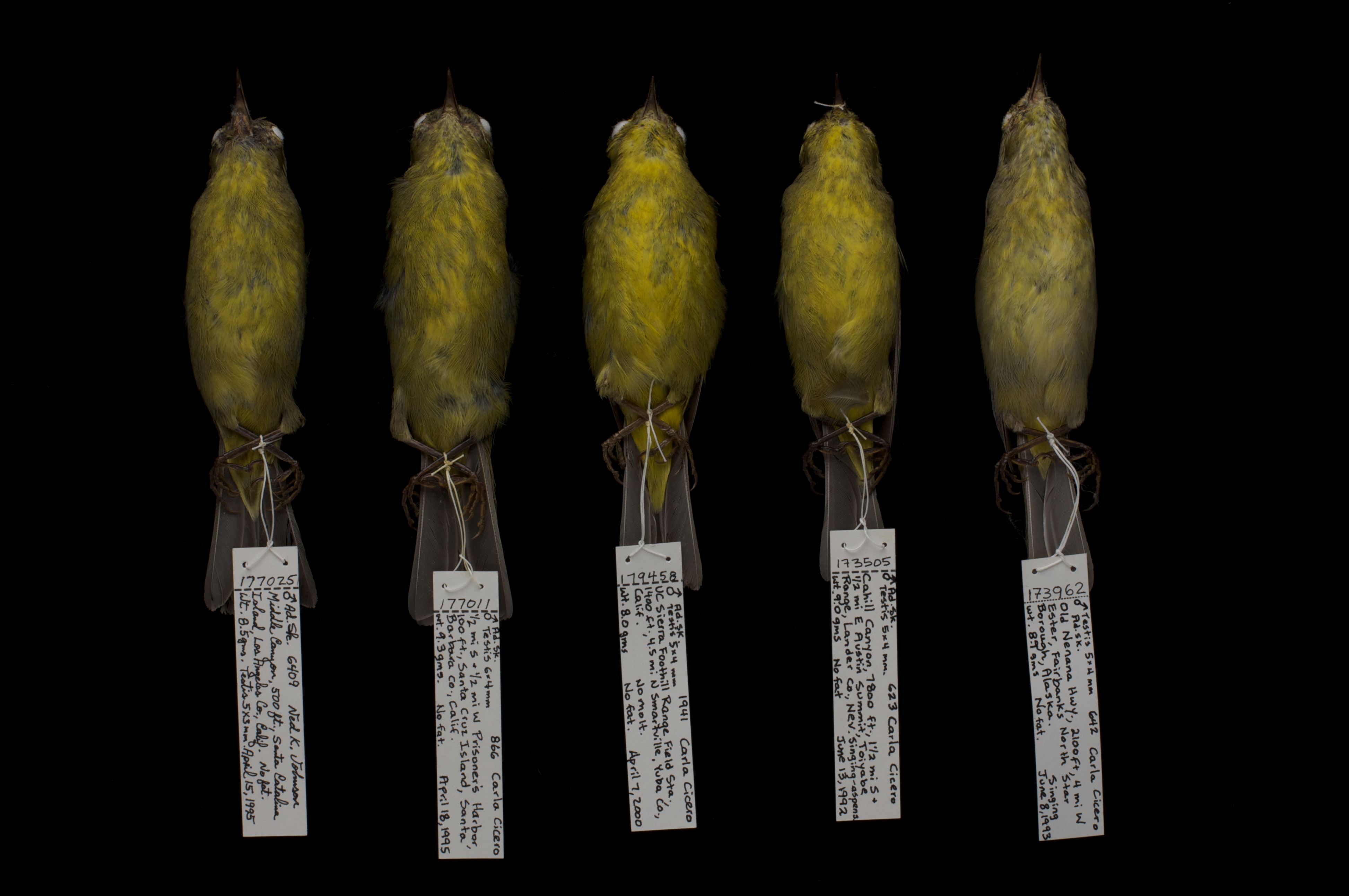
Ventral specimen photos
This is a ventral view of five Oreothlypis celata museum skins. From left to right, the specimens are MVZ:Bird:177025, MVZ:Bird:177011, MVZ:Bird:179458, MVZ:Bird:173505, and MVZ:Bird:173962. These represent the four recognized subspecies with representatives of O. c. sordida from both the southern and northern Channel Islands. From left to right, the specimens are an O. c. sordida from Santa Catalina Island; an O. c. sordida from Santa Cruz Island; an O. c. lutescens from interior northern California; an O. c. orestera from Nevada; and an O. c. celata from Fairbanks, Alaska. Image taken by Anand Varma, reproduced with permission.
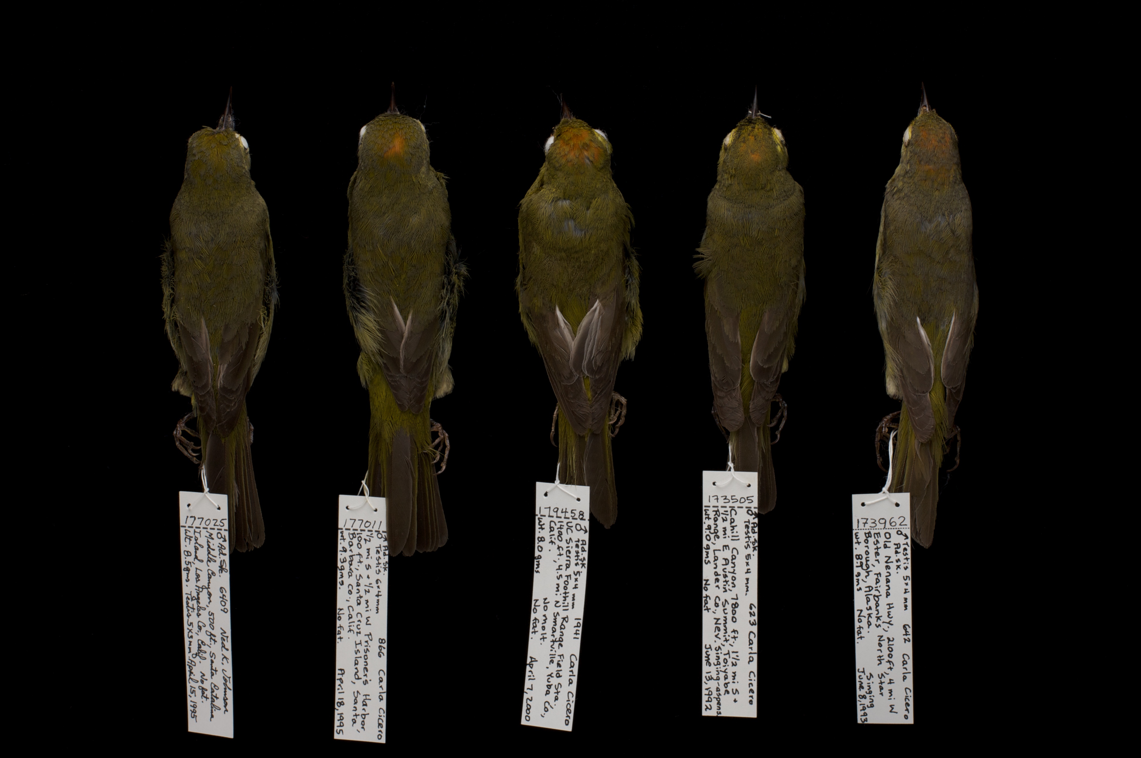
Dorsal specimen photos
This is a dorsal-view of the same five specimens seen in Fig. S1. Image taken by Anand Varma, reproduced with permission.
ND2 haplotype network with coast-interior population grouping
This is the ND2 haplotype network colored by samples’ grouping into coast and interior populations. See Fig. 3 for the haplotype numbers that correspond with the numbers in Table S1. The size of each circle is proportional to the number of individuals with that haplotype. Lines connect haplotypes that differ by one mutation. Dots represent inferred haplotypes. Hash marks indicate the number of mutations between haplotypes separated by more than one mutation.
Structure plot for K =2 with Channel Islands population excluded
This figure depicts the ancestry of each individual in the two genetic clusters identified by Structure within the seven labeled populations after we excluded the Channel Islands population. Different colors represent the two genetic clusters identified by Structure. Each vertical bar represents an individual Oreothlypis celata. The height of each color in a given bar illustrates the proportion of ancestry derived from each genetic cluster for that individual.