
Population genetics and historical demographic inferences of the blue crab Callinectes sapidus in the US based on microsatellites
- Published
- Accepted
- Received
- Academic Editor
- James Reimer
- Subject Areas
- Aquaculture, Fisheries and Fish Science, Genetics, Marine Biology
- Keywords
- Population genetics, Marine connectivity, Microsatellites, Crustaceans, Blue crab, Extended pelagic larval duration, Gulf of Mexico, Fisheries, Keystone species, Genetic diversity
- Copyright
- © 2019 Macedo et al.
- Licence
- This is an open access article distributed under the terms of the Creative Commons Attribution License, which permits unrestricted use, distribution, reproduction and adaptation in any medium and for any purpose provided that it is properly attributed. For attribution, the original author(s), title, publication source (PeerJ) and either DOI or URL of the article must be cited.
- Cite this article
- 2019. Population genetics and historical demographic inferences of the blue crab Callinectes sapidus in the US based on microsatellites. PeerJ 7:e7780 https://doi.org/10.7717/peerj.7780
Abstract
The native range of the blue crab Callinectes sapidus spans Nova Scotia to northern Argentina. In the US, it constitutes a keystone species in estuarine habitats of the Atlantic coast and Gulf of Mexico (GOM), serving as both predator and prey to other species, and also has historically represented a multi-billion dollar fishery. Knowledge relevant to effective management and monitoring of this ecologically and economically important species, such as levels of population genetic differentiation and genetic diversity, is necessary. Although several population genetics studies have attempted to address these questions in one or more parts of its distribution, conflicting results and potential problems with the markers used, as well as other issues, have obscured our understanding on them. In this study, we examined large-scale genetic connectivity of the blue crab in the US, using 16 microsatellites, and genotyped individuals from Chesapeake Bay, in the US Atlantic, and from nine localities along the US GOM coast. Consistent with the high long-distance dispersal potential of this species, very low levels of genetic differentiation were detected for the blue crab among the ten US localities examined, suggesting it constitutes a large panmictic population within this region. Estimations of genetic diversity for the blue crab appear to be high in the US, and provide a baseline for monitoring temporal changes in this species. Demographic analyses indicate a recent range expansion of the US population, probably during the Holocene. In addition, capitalizing on published microsatellite data from southern Brazil, our analyses detected high genetic differentiation between localities in the US and Brazil. These results point to the need for examination of genetic diversity and differentiation along the area spanning the US to southern Brazil.
Introduction
The blue crab Callinectes sapidus Rathbun, 1896, whose natural range spans from Nova Scotia to northern Argentina (Williams, 1984), is an estuarine keystone species that plays a crucial role in the estuarine food web as both predator and prey. Blue crabs are opportunistic foragers that feed on a variety of organisms that include other crustaceans, gastropods, fish, bivalves, algae, vascular plants, zooplankton, infauna, as well as detritus (Alexander, 1986; Fitz & Wiegert, 1991; Laughlin, 1982; Meise & Stehlik, 2003; Rosas, Lazaro-Chavez & Bückle-Ramirez, 1994). The blue crab can regulate the abundance of some of its prey populations, which can have drastic effects on the whole estuarine ecosystem (Eggleston, 1990; Mansour & Lipcius, 1991; Silliman & Bertness, 2002). As a prey, the blue crab is one of the main food items of the critically endangered whooping crane during its winter migration period in south Texas (Hunt & Slack, 1989), and reductions in the abundance of blue crabs appear to be correlated with increased mortality of whooping cranes during this period (Pugesek, Baldwin & Stehn, 2013; Stehn, 2001, 2011). Blue crabs also constitute an important prey item of the critically endangered Kemp’s Ridley sea turtle (Burke, Morreale & Standora, 1994; Seney, 2016; Witzell & Schmid, 2005), as well as of commercially important fish species, such as the red drum (Scharf & Schlicht, 2000).
The blue crab also has historically represented a multi-billion dollar fishery in the US; constituting an important economic activity in the US Middle Atlantic, South Atlantic and Gulf of Mexico (GOM) regions. In 2016 alone, 74,258 metric tons were caught in the US, worth ~$214 million (NOAA, 2018). Large local reductions of blue crabs, however, appear to have occurred in some areas, as suggested by the sharp decline in the landings of this crab in recent years, such as in the Texas coast (NOAA, 2018). Due to the ecological and commercial importance of the blue crab in the US, it is crucial to obtain information that can aid its management and monitoring, such as population genetic differentiation, genetic diversity, and demographic history (reviewed in Hauser & Carvalho, 2008).
Long-distance dispersal, and thus, low levels of genetic differentiation at large geographical scale, may be expected for the blue crab due to its extended pelagic larval duration that ranges for 4–7 weeks, followed by a postlarval megalopal stage of 1–3 weeks (Costlow & Bookhout, 1959). Thus, oceanic circulation can contribute to the dispersal of larvae and megalopae away from their parent estuaries (Epifanio, 1995; Epifanio, Valenti & Pembroke, 1984). Gene flow, however, can be affected by variation in environmental factors (e.g., salinity, temperature), as well as potential barriers for dispersal. Genetic breaks for marine species have been observed at: north vs. south of Cape Canaveral; between the Atlantic and GOM; East vs. West GOM; and between the Laguna Madre and other GOM localities (Avise, 2000; Hollenbeck, Portnoy & Gold, 2019 and references therein; Milá et al., 2017; Neigel, 2009).
Previous large-scale studies of population genetic differentiation of the blue crab in the US have been conducted using allozymes, mitochondrial restriction fragment length polymorphisms (RFLPs) and sequences, and nuclear protein-coding genes sequences. The degree of connectivity of the blue crab in its US range, however, remains uncertain, due to conflicting results among studies. Several sources of bias or lack of power (e.g., insufficient number of markers, limited genetic variability of markers, inherent limitations of markers, small sample sizes, and potential species misidentifications) could have affected one or more of these studies.
On the basis of three moderately polymorphic allozymes, a study conducted in the Texas coast reports significant spatial and temporal population genetic differences in megalopa and adult samples (Kordos & Burton, 1993). Other allozyme-based studies, however, examining a considerably higher number of allozymes, suggest panmixia within the GOM and in the US range of this species (Berthelemy-Okazaki & Okazaki, 1997; McMillen-Jackson, Bert & Steele, 1994). Moreover, genetic differences detected among megalopa populations in the Texas study could be due to misidentifications between C. sapidus and C. similis (Sullivan & Neigel, 2017). According to Sullivan & Neigel (2017), the morphological characters used by Kordos & Burton (1993) to distinguish megalopae of both species are not diagnostic. In addition, Sullivan & Neigel (2017) found a temporal composition shift in the abundance of C. similis and C. sapidus megalopae that parallels changes in the allozyme allele frequencies reported for blue crab megalopae at the same localities studied by Kordos & Burton (1993). On the other hand, inferences of genetic homogeneity in the McMillen-Jackson, Bert & Steele (1994) and Berthelemy-Okazaki & Okazaki (1997) studies may correspond to overestimates of gene flow from broad scale stabilizing selection acting at the allozyme loci surveyed (Karl & Avise, 1992).
McMillen-Jackson & Bert (2004) used RFLP analysis of the mitochondrial DNA to examine patterns of genetic variation in blue crab populations distributed from New York to the southern GOM, and found no geographic structuring. Darden (2004), however, based on variation in mitochondrial Cytochrome C Oxidase Subunit I (COI) sequences in localities along the GOM coast, reports differences between the eastern and western GOM, and among some localities within the western GOM. Based on Darden (2004), the Gulf States Marine Fisheries Commission proposed two blue crab stocks for management within the US GOM, with their division around Apalachicola, Florida (reviewed in Perry & VanderKooy, 2015). Nonetheless, a more recent study that examined variation in mitochondrial NAD2 sequences for blue crab samples collected from Massachusetts to Texas reports a lack of geographic genetic structure (Feng, Williams & Place, 2017). Mitochondrial markers, however, appear particularly problematic for inferring population connectivity and genetic diversity in the blue crab, as extremely high levels of mtDNA heteroplasmy have been recently reported in this species. Based on polymerase chain reaction (PCR), cloning, and sequencing of segments of the ND2, ND4, and COI mitochondrial loci, Williams, Feng & Place (2017) detected as many as 24 NAD2 haplotypes in a single individual (for which 17 COI haplotypes were also observed), and the dominant haplotype accounted for as little as 43.9% of the total sequences observed within an individual.
High levels of gene flow are reported in the northern GOM, between localities in the Louisiana coast and the Lower Laguna Madre, Texas, based on sequences of four nuclear protein-coding genes (Yednock & Neigel, 2014b), three of which show signatures of selection (Yednock & Neigel, 2014a). Nonetheless, significant temporal differences were found for adults between 2 years at the four genes within a single Louisiana location.
Despite being one of the most widely used markers to examine genetic connectivity in animals (Allendorf, 2017), including marine invertebrates (Selkoe et al., 2016), large-scale microsatellite-based studies are lacking for the blue crab within the US. Microsatellites usually show high levels of genetic diversity, and there is a good understanding of their use in population genetics, as well as the availability of extensive tools for their analyses (Allendorf, 2017; Selkoe & Toonen, 2006). A seemingly limited number of microsatellites, however, have been reported for the blue crab: eight highly polymorphic microsatellites (although one pair was reported in linkage disequilibrium (LD)) were developed from a blue crab individual in Chesapeake Bay, where they were shown to be highly variable (Steven et al., 2005). A set of six of these microsatellites was used to examine genetic diversity of blue crabs in Charleston Harbor, South Carolina, where they were also highly variable (Cushman & Darden, 2017). In addition, a set of seven of these microsatellites was used in a study that determined a lack of genetic differentiation for this species along a 740 Km stretch in southern Brazil (Lacerda et al., 2016). Although these microsatellites are, in general, highly diverse in the three regions where they have been used, studies of genetic differentiation in the blue crab may benefit from the addition of other polymorphic microsatellites.
Herein, we developed nine new polymorphic microsatellites for the blue crab and examined population genetic differentiation in individuals collected from nine localities along the US GOM and in the Chesapeake Bay using a total of 16 microsatellite markers. We also estimated genetic diversity and effective population size, and examined historical demography. Finally, we capitalized on a published microsatellite dataset from southern Brazil (Lacerda et al., 2016), and tested genetic differentiation and compared genetic diversity between blue crabs in that region and our study area.
Materials and Methods
Samples
Adult blue crabs were collected in the US from nine localities across the GOM and one in the Chesapeake Bay (Fig. 1). Specimens were assigned to C. sapidus on the basis of diagnostic traits (Williams, 1974, 1984). Eight localities were sampled in 2014: Rockport (ROC; n = 24); Port Lavaca (POL; n = 18); Galveston (GAL; n = 12); Avery Island (AVI; n = 20); Slidell (SLI; n = 11); D’Iberville (DIB; n = 24); Apalachicola (APA; n = 21); and Cedar Key (CEK; n = 13). Lower Laguna Madre (LLM; n = 24) and Chesapeake Bay (SERC; n = 25) were sampled in 2015. In seven GOM localities, crabs were sampled using double ring mesh nets with chicken as bait. In Rockport and D’Iberville, live crabs were purchased from local fishermen. Crabs from Chesapeake Bay were sampled by Midge Kramer (Smithsonian Environmental Research Center). Sampled crabs were stored in a cooler with dry ice, when available, or regular ice. A chela from each crab was dissected and stored in 100% ethanol for DNA preservation.
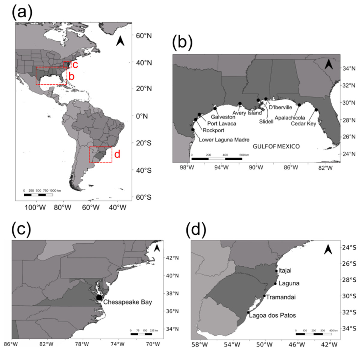
Figure 1: Sampling localities.
(A) All sampling locations for this study (in the US) and from Lacerda et al. (2016) in southern Brazil. (B) Sampling locations in the Gulf of Mexico. (C) Sampling location in Chesapeake Bay. (D) Sampling locations from Lacerda et al. (2016) in southern Brazil.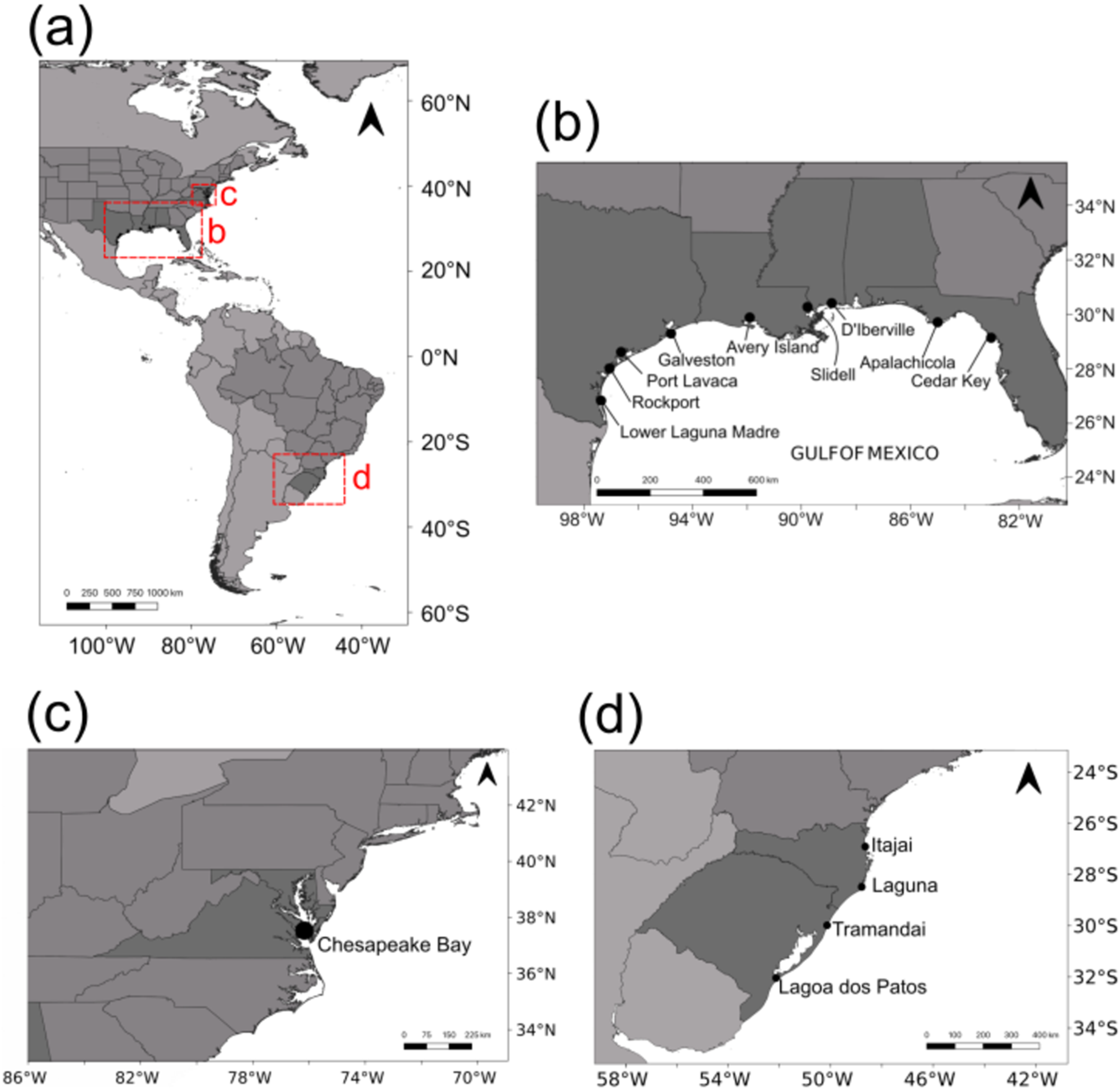
Molecular methods
DNA was extracted from muscle tissue dissected from the chela with Quick-gDNA™ MiniPrep kit (Zymo Research Corporation, Irvine, CA, USA), according to the manufacturer’s “Solid Tissue” instructions. DNA quality was visually checked following electrophoresis on a 2% agarose gel stained with 0.1× GelRed (Biotium, Inc., Hayward, CA, USA).
For each individual, amplifications of a total of 16 microsatellites were attempted using the PCR. Nine of these (first nine in Table S1) were newly developed, whereas the remaining markers (last seven in Table S1) were reported by Steven et al. (2005) and used by Lacerda et al. (2016). PCRs were performed following the method of Schuelke (2000). For the newly developed microsatellites, an M13 universal tag sequence was added to the 5′-end of the forward primers (5′-TGTAAAACGACGGCCAGT-3′) and a seven-bp pigtail was added to the 5′-end of the reverse primers (5′-GTGTCTT-3). The addition of the pigtail forces non-template adenosine to be added to the 3′ end, thus helping reduce genotyping error (Brownstein, Carpten & Smith, 1996; Harker, 2001). The pigtail, however, was not added to the seven loci that were also used by Lacerda et al. (2016) to avoid discrepancies in allele calling between studies (see below). To insert a fluorescent dye into each reaction, a third M13 universal primer labeled with 6-FAM™, HEX™, or NED™ was added (Integrated DNA Technologies, Coralville, IA, USA; Applied Biosystems, Foster City, CA, USA).
Due to the varying degree of amplification success for each marker, different PCR reaction mixes were utilized. The seven markers (i.e., CSA121, CSC094, CSA073, CSC007, CSC001, CSA035, and CSC004) reported by Steven et al. (2005) and used by Lacerda et al. (2016) were amplified using the Type-It Microsatellite PCR Kit (QIAGEN, Valencia, CA, USA). Each five μL reaction contained 1× Type-It Multiplex PCR Mastermix, 1× Q Solution, 1.25 μM of the forward primer, five μM each of the reverse and M13 primers, and 40–150 ng DNA. The PCR reactions were performed on a BioRad MyCycler (Biorad, Hercules, CA, USA). They began with a denaturing step at 95 °C for 5 min, followed by 28 cycles of denaturation at 95 °C for 30 s (s), annealing at 44–58 °C for 90 s (see Table S1), and extension 72 °C for 30 s. An additional 10 cycles were used to embed the fluorescent dye, at 94 °C for 30 s, 53 °C for 45 s, and 72 °C for 45 s. A final extension at 60 °C for 30 min was used.
The nine new microsatellite loci were amplified with PCR reactions containing 40–150 ng DNA; 1× PCR buffer; 1 U Taq DNA polymerase (New England BioLabs, Inc., Ipswich, MA, USA); 1.25 μM forward primer; five μM of reverse and fluorescent M13 universal primer; 200 μM of each dNTP, for a final volume of 15 μL. The marker Pen23472 had 1.6 mM MgCl2 added to each reaction. The thermocycler conditions consisted of: a denaturation step at 95 °C for 5 min, followed by 30 cycles of 95 °C for 30 s, 53–63 °C for 35 s (see Table S1), and extension at 72 °C for 30 s. The same 10 cycles used above were included for incorporation of the fluorescent dye. A final extension at 72 °C for 10 min was used.
Following PCR, samples were prepared for genotyping by diluting one μL of PCR products into 8.7 μL of formamide and 0.3 μL of MapMarker-ROX size standard (BioVentures, Inc., Murfreesboro, TN, USA). These were subsequently analyzed on an ABI 3130x1 Genetic Analyzer at the DNA Technologies Lab and Institute for Plant Genomics at Texas A&M University. Two researchers (DM and ICC) independently performed allele calling with GeneMarker v.1.6 (Softgenetics, State College, PA, USA) and STRand v.2.4.109 (Toonen & Hughes, 2001), respectively. Reproducibility and scoring consistency was assessed by randomly selecting 30% of the samples and repeating PCR amplification and genotyping. Negative controls (with water instead of DNA template) were included in all PCR reactions.
Genetic analyses
Basic tests, genetic diversity, inbreeding and relatedness
PGDSpider v. 2.1.0.3 was used to convert data files between software packages (Lischer & Excoffier, 2012). GENEPOP on the Web 4.6 (Raymond & Rousset, 1995; Rousset, 2008) was used to test LD, estimate expected and observed heterozygosity (HE, HO), test conformity to the expectations of Hardy-Weinberg Equilibrium proportions (HWP), and calculate FIS for each marker. To control for the occurrence of false positives due to multiple comparisons, significance of LD and HWP p-values was determined using: (1) the Bonferroni correction; and (2) the Benjamini–Hochberg procedure (Benjamini & Hochberg, 1995) at a false discovery rate (FDR) of 0.01 and 0.05. All GENEPOP analyses were performed with a dememorization number of 5,000, 500 batches, and 5,000 iterations per batch. Mean observed heterozygosity within populations (HO), mean expected heterozygosity within populations (HS), total heterozygosity (HT), inbreeding coefficient (GIS), allelic richness (AR), and number of alleles (NA) for each locus and group were measured with FSTAT v.2.9.3.2 (Goudet, 1995). The number of private alleles (NP) per locus was determined in GenAIEx v. 6.5 (Peakall & Smouse, 2006, 2012).
MICRO-CHECKER v. 2.2.3 (Van Oosterhout et al., 2004) was used to check for the potential presence of null alleles and scoring errors. As presence of null alleles can lead to false excess of homozygosity, and thus, overestimation of inbreeding, a Bayesian approach implemented in INEST ver. 2.1 (Chybicki & Burczyk, 2009) was used to obtain unbiased multilocus estimates of the inbreeding coefficient (f) while accounting for null alleles (n), allelic dropout (b) and inbreeding (f). INEST was initially run using the six models available, with 50,000 burn-in cycles and 500,000 cycles overall, to determine the best models for our dataset, according to the deviance information criterion (DIC). The best models were then run to 1,000,000 cycles with 100,000 burn-in cycles. Mean paired genetic relatedness values (r) within each locality were estimated using allele frequencies according to the mean estimate (r), as described by Queller & Goodnight (1989), and implemented in GenAlEx 6.5. A total of 9,999 permutations were run to generate a null distribution of r values on which the computed r was compared to assess its significance, and 10,000 bootstrap replicates were run to obtain 95% confidence intervals (CI) for each r.
Genetic diversity estimations obtained for US localities were compared with those obtained by Lacerda et al. (2016) for Brazil using seven loci common between the two studies. To evaluate how sample size may affect AR, a rarefaction analysis was performed in Allelic Diversity Analyzer v. 1.0 (ADZE; Szpiech, Jakobsson & Rosenberg, 2008).
Presence of loci under putative selection was tested with the method of Beaumont & Nichols (1996) implemented in the program ARLEQUIN v.3.5.2.1 (Excoffier & Lischer, 2010). This method performs coalescent simulations to estimate the distributions of heterozygosity and FST under the island model. Loci that do not fit neutral expectations are considered candidates of selection. Simulations assumed 100 demes with 20,000 simulated loci. Analyses were conducted considering either ten groups (i.e., each population corresponds to a group) or three groups (i.e., the Atlantic locality (SERC), the eastern GOM (APA, AVI, CEK, DIB, SLI), and the western GOM (GAL, POL, ROC, LLM)). The Bayesian simulation-based test of Beaumont & Balding (2004), implemented in the software Bayescan v.2.1 (Foll & Gaggiotti, 2008), was also used to detect the presence of loci under putative selection. This method decomposes FST values into locus-specific components (α) and population-specific components (β). It uses a reversible jump Markov Chain Monte Carlo (MCMC) algorithm and calculates the posterior probability that a locus is under selection by assuming two alternative models (selection-based model and neutral model). Analyses were based on 20 pilot runs, each consisting of 5,000 iterations, followed by 100,000 iterations with a burn-in of 50,000 iterations.
Population genetic differentiation
The statistical power of the datasets used for detecting population structure was evaluated using POWSIM v. 4.1 (Ryman & Palm, 2006). For each test, 1,000 runs/simulations were performed at four levels of population genetic differentiation and 10 generations (t): FST = 0.01 (Ne = 500, t = 10), FST = 0.007 (Ne = 750, t = 10), FST = 0.005 (Ne = 1,000, t = 10), and FST = 0.001 (Ne = 5,000, t = 10).
Jost’s differentiation (DST), which quantifies relative degree of allelic differentiation, and fixation index (GST), which quantifies nearness to fixation, were calculated using FSTAT. Population differentiation was also estimated using FST, another measure that quantifies nearness to fixation, calculated in GenAlEx, GENODIVE (Meirmans & Van Tienderen, 2004), and FreeNA (Chapuis & Estoup, 2007). FST results from FreeNA were obtained with and without corrections for null alleles. FreeNA does not calculate p-values per se, but provides 95% CI for FST. Therefore, CI’s that excluded zero were deemed statistically significant. p-values for uncorrected FST were estimated using Arlequin v.3.5.2.2 (Excoffier & Lischer, 2010), with 10,000 permutations and the Benjamini-Hochberg procedure; FDR values ≤ 0.05 were deemed statistically significant.
FST was also estimated using the private alleles method (Barton & Slatkin, 1986), as implemented in Arlequin. Recent migration rates (over the last several generations) were estimated between localities using a MCMC framework implemented in BayesAss BA3 v.3.0.4 (Wilson & Rannala, 2003). Values were estimated after 5,000,000 burnin steps to allow for convergence out of 50,000,000 iterations, sampling every 5,000 iterations. Mixing parameter values for allele frequency (-a), inbreeding coefficient (-f), and migration rate (-m) were set to 0.8. This value was selected after performing preliminary runs implementing different mixing parameter values (0.2 through 0.8), and examining the acceptance rates and mixing patterns of the chains (visualized in Tracer v.1.7). Multiple runs and the convergence of chains were checked by plotting traces in Tracer v.1.7. The method implemented in BayesAss assumes migration rates are relatively low and the proportion of non-migrants within a population (locality) is bound at a minimum of 2/3. Estimated non-migration rates of approximately 2/3 may indicate that the actual value is lower than this, suggesting that populations may not be distinct (BayesAss 1.3 Documentation).
Locus-by-locus analyses of molecular variance (AMOVA) and significance tests with 10,000 permutations were also performed in Arlequin. The data were grouped in multiple ways to examine patterns of variation: (1) all US localities; (2) all GOM localities; (3) GOM and Chesapeake Bay grouped separately; and (4) western and eastern GOM grouped separately.
STRUCTURE 2.2.3 (Pritchard, Stephens & Donnelly, 2000), which performs model-based clustering with a Bayesian approach, was used to examine population subdivision. K values from 1 to 10 were tested in three iterations, with 500,000 steps and a burn-in of 125,000 steps. Four models were used: admixture with correlated allele frequencies; admixture with independent allele frequencies; no admixture with correlated allele frequencies; and no admixture with independent allele frequencies. All other settings were set to default. Values of Ln Pr(X|K) (Pritchard, Stephens & Donnelly, 2000), ΔK using the Evanno method (Evanno, Regnaut & Goudet, 2005), and MedMedK, MedMeaK, MaxMedK, and MaxMeaK (Puechmaille, 2016), which are used to explore the number of K, were estimated using Structure Selector (Li & Liu, 2018). The LOCPRIOR setting in Structure (Hubisz et al., 2009), which is suggested in cases of weak structure, was also used to estimate clustering membership, conducting analyses for the admixture and non-admixture models with correlated allele frequencies for K values between 2 and 10, with five iterations for each model. The LOCPRIOR setting is useful in cases where: samples come from different populations; FST pairwise values between these populations are significantly different from zero; and yet results based on the default model in STRUCTURE indicate no evidence of structure. Appropriateness for using the LOCPRIOR setting was checked by assessing r, a parameter that estimates the informativeness of the sampling location data. Values of r >> 1 imply locations are non-informative about ancestry, whereas values of r near or below 1 imply that the ancestry proportions vary considerably between locations.
The program TESS 2.3.1 (François, Ancelet & Guillot, 2006) was also used to examine population subdivision. This program implements a Bayesian clustering algorithm for spatial population genetic studies, searching for population structure from individual multilocus genotypes sampled at distinct geographical locations without assuming predefined populations. TESS analyses were run for Kmax ranging from two to five for 50,000 sweeps, discarding the first 10,000 sweeps, and each K was repeated five times. A discriminant analysis of principal component analysis (DAPC) with the R package adegenet v.2.1.1 (Jombart, 2008; Jombart & Ahmed, 2011) also was used to examine potential population differentiation. DAPC is a non-model-based method that maximizes the differences between groups while minimizing variation within groups (Jombart, Devillard & Balloux, 2010). No prior information on population groups was assumed, and the function find.clusters was applied to assess the optimal number of groups based on the Bayesian information criterion method. In addition, GenAlEx was used to construct a genetic distance matrix, from which a principal coordinate analysis (PCA) was performed to identify population clusters. Finally, GENETIX v. 4.05 (Belkhir et al., 2004) was used to conduct a three-dimensional factorial correspondence analysis (FCA). This method seeks to identify correspondence between values in rows and columns, such as individuals and alleles.
Analyses of Isolation by distance (IBD) within the US and GOM were conducted using the program ISOLDE in Genepop on the Web. Two kinds of analyses were performed: (1) between localities, and (2) between individuals. Geographic distances were estimated in Google Earth Pro v.7.3 following the contours of the coastal margin between localities. Statistical significance based on the Spearman’s rank correlation coefficient was evaluated using Mantel tests (Mantel, 1967).
The aforementioned set of analyses of population genetic differentiation (except IBD) were also conducted on the genotypic data of the study by Lacerda et al. (2016) from southern Brazil, and our genotypic data including only the seven common microsatellites between both studies. Genetic diversity of blue crabs between the US and Brazil was also compared.
Effective population size and bottlenecks
Effective population size (Ne) was estimated with NeEstimator v. 2.01 (Do et al., 2014) using the LD and heterozygote excess methods. BOTTLENECK v. 1.2.02 (Piry, Luikart & Cornuet, 1999) was used to search for signatures of a recent bottleneck (i.e., higher heterozygosity than that expected at mutation-drift equilibrium) in the blue crab populations. A Wilcoxon’s test was conducted for the three possible mutation models: infinite allele model (IAM), stepwise mutation model (SMM), and the two-phase model (TPM). For TPM, the model suggested for microsatellites, it is recommended to use 95% single-step mutations and 5% multi-step mutations, as well as a variance of 12 among multiple steps (Piry, Luikart & Cornuet, 1999). BOTTLENECK also examines the allele frequency distribution. Under mutation-drift equilibrium, an L-shaped distribution is expected, whereas a recent bottleneck is expected to cause a mode shift.
Population demographic history was also examined with MIGRAINE v0.5.1 (Rousset, Beeravolu & Leblois, 2018). Based on the population genetic differentiation results (see “Results” section), a model of a single panmictic population with a single past change in population size was assumed (OnePopVarSize, Leblois et al., 2014). One analysis was conducted with seven loci, referred to as the US-seven-loci-dataset (see “Results” section). A generalized stepwise mutation model (GSM) was used for this analysis, which reduces the risk of false positives when testing for a bottleneck. Two additional analyses were conducted with a 15-loci dataset (i.e., removing one locus that appears to be under selection; see “Results”). One of these analyses used the GSM model, and the other a combination of the GSM model for di-nucleotides and a strict SMM for tri-, tetra-, and penta-nucleotide motifs. The combined model accommodates different mutation rates for microsatellites with various motifs. For each analysis, MIGRAINE was run for a total of five iterations, each using 2,000 points, with 20,000 trees per point. Point estimates with their corresponding 95% CI were obtained for the following parameters: pGSM, which is the parameter of a geometric distribution determining the mutation size in number of repeats; θcur (2Nμ), which is the current effective population size; θanc (2Nancμ), which is the ancestral effective population size; Dg/2N, where Dg is the time of the demographic change in generations and N is the effective population size; and Dg * μ, where μ is the mutation rate per generation per locus. Inferences on population contraction or expansion are based on the Nratio (θcur/θanc), which is the ratio of the current effective population size divided by the ancestral one; a ratio > 1 is interpreted as a signal of population expansion, whereas a ratio < 1 as a signal of a bottleneck. Unscaled parameters of N, Nanc, and Dg were converted using a microsatellite mutation rate of 0.0005 per locus per generation, which represents a classical average value derived from many different species (Estoup & Angers, 1998; Goldstein & Schlotterer, 1999).
Results
Basic tests and genetic diversity estimations
Genotyping scores for all individuals are shown in Dataset S1. Reproducibility was 100% for all the samples that were repeated (30% of the total samples). LD was not detected among loci after Bonferroni correction (p < 0.0005), nor with the BH FDR method (FDR ≤ 0.05). Both selection tests identified locus Pen23472 as an outlier, suggesting it may be under putative selection (Fig. S1).
Table S2 shows genetic diversity estimations and inbreeding coefficients (FIS) per locus for each of the 10 US localities (16 loci). For comparison, we also show these data for the four Brazilian localities (from Lacerda et al., 2016). Percentage of private alleles in relation to the total number of alleles observed per locality in the US was low (calculated from values shown in Table S2), ranging from 2.6% to 5.2% (average 2.96%); whereas in Brazilian localities ranged from 4.4% to 12.7% (average 8.95%).
For the 15 putatively neutral loci (i.e., excluding Pen23472), no significant deviations from HWP were detected in 10 of them at any US locality after Bonferroni correction (p < 0.0003), whereas two loci (Tri24376 and Tet1886) showed deviations of HWP in only one locality, one locus (CSA035) in three localities, and two loci (CSC004 and CSC001) in five localities (Table S2). Using the BH FDR method with FDR ≤ 0.01, 37 tests resulted in significant deviations of HWP. No significant deviations of HWP were detected in six of the 15 putatively neutral loci: Tet6290, Tet1329, Tet603, CSA121, Di680, and CSC094. For CSA073, Pen9028 and CSC007, significant deviations of HWP were observed in only one locality. For the remaining loci, deviations of HWP were found in two to seven localities. Using a FDR ≤ 0.05, 63 tests resulted in significant deviations of HWP. No significant deviations of HWP were suggested in Tet6290, Tet1329, Tet603, and CSA121. For CSC094 and CSA073, significant deviations of HWP were found only in one locality, for Di680 in three localities, and for the remaining loci in four to nine localities. MICRO-CHECKER did not suggest the presence of potential null alleles at any locality for Tet6290, Tet1329, Tet603, Pen23472, and CSA121. For Di680 and CSC094, null alleles were only suggested in one locality, and for CSA073 in two localities. For the remaining eight loci, null alleles were suggested in four to 10 populations (Table S2). Pooling data from all US localities (i.e., treating the dataset as a single panmictic population; see genetic differentiation results), no significant deviations from HWP were observed in six of the neutral loci: Tet6290, Tet1329, Tet603, CSA121, Di680, and CSC094. MICRO-CHECKER analyses with pooled data did not suggest the presence of potential null alleles in five of these loci: Tet6290, Tet1329, Tet603, CSA121, and CSC094 (Table S3). A low percentage of null alleles was suggested for Di680 (5%) and CSA073 (4%).
The number of alleles per locus for the 16 loci in the US ranged from six to 47; average 18.1 (Table S3). Percentage of missing data per locus ranged from 0.0% (Tet1329) to 11.3% (Tet1886), with an overall average of 3.7% (Table S3). Average mean observed (HO) and expected heterozygosity (HS) per locus within localities was 0.59 and 0.73, respectively (Table S3). Average total expected heterozygosity (HT) per locus in the US was 0.74.
For comparison, allelic range and average alleles per locus in the Brazilian localities were 3–43 and 26.0, respectively (Table S3). These values are similar to those observed in the US localities for the seven common loci between the two studies: 7–47 allelic range and 28.1 average alleles per locus. Marked differences in HS were observed for all but one (CSC007) of the loci in common between the US and southern Brazil. Average HO, HS and HT in Brazil was 0.54, 0.58, and 0.58, respectively (Table S3); whereas these values in the US for the seven common loci between the two studies were 0.63, 0.82, and 0.82, respectively. Rarefaction analyses conducted in ADZE suggest that the sample sizes used captured most of the allelic diversity present in both regions, ~91% for the 16 loci in the US (Fig. S2).
Inbreeding and relatedness
Among the 15 putatively neutral loci, the lowest inbreeding coefficients were estimated for the seven loci that showed the least deviations of HWP and least presence of null alleles (i.e., Tet6290, Tet1329, Tet603, CSA121, CSC094, Di680, and CSA073), hereafter referred to as the “US-seven-loci-dataset” (Table S3). Because null alleles were either not detected or detected at low frequency for these loci, we do not expect inbreeding estimations for them to be largely biased (null alleles can inflate homozygosity and thus inbreeding estimations). Average GIS for all US populations for these seven loci was 0.02. Average GIS for the remaining eight loci was 0.34, but these values are likely upwardly biased due to the presence of null alleles (see INEST results below), which were suggested in four or more populations. GIS estimation for the outlier locus Pen23472 was −0.040 (Table S3). Pooling data from all US localities (i.e., treating the US dataset as a single panmictic population), average FIS for the US-seven-loci-dataset is 0.015. INEST results correcting for null alleles, genotyping failures and inbreeding also indicate very low inbreeding. Pooling data from all localities for the 15 neutral loci, the best models were nb (null alleles and genotyping failures) and nfb (null alleles, inbreeding coefficients, and genotyping failures), with DIC values of 19,383.164 and 19,384.124, respectively; and their estimated inbreeding coefficients were 0 and 0.021, respectively. Of the two models, the best one was nb (null alleles and genotyping failures), implying that inbreeding was not important. Mean paired genetic relatedness values (r) within each locality were very low (Fig. S3), ranging between 0.035 in Apalachicola and −0.040 in Cedar Key (average −0.0023), and none were significant (i.e., all fell within the 95% CI).
Population genetic differentiation within the US
Within the US, very low global DST (Jost’s differentiation) and GST (fixation index) values were obtained for each locus, with the exception of Pen23472, which was suggested to be under putative selection (Table S4). Global average corrected DST′ (measure of allelic differentiation) and GST′ (measure of fixation) values per locus for the US-seven-loci-dataset, which contains the seven loci that exhibited the least deviations of HWP and the least presence of null alleles, were 0.004 and 0.006 respectively. Global average corrected DST′ and GST′ values per locus for the 15 putatively neutral loci (i.e., excluding Pen23472) were 0.002 and 0.004 respectively. In contrast, corrected global DST′ and GST′ values for the outlier locus Pen23472 were higher: 0.049 and 0.062, respectively.
Using the US-seven-loci-dataset and correcting for null alleles, average pairwise FST was 0.008 (estimated from values in Table 1). In this analysis, the 95% CI of four of the 45 pairwise FST comparisons excluded zero: Apalachicola vs. Avery Island (FST = 0.009; CI [0.004–0.014]); Apalachicola vs. D’Iberville (FST = −0.008; CI [−0.014–0.002]); Cedar Key vs. Galveston (FST = 0.025; CI [0.003–0.046]); and Galveston vs. Lower Laguna Madre (FST = 0.014; CI [0.0004–0.027]). Without correction for null alleles, average pairwise FST estimations was 0.006. In this analysis, three pairwise comparisons did not include zero in the 95% CI: Apalachicola vs. D’Iberville (FST = −0.008; CI [−0.014 to −0.002]); Cedar Key vs. Galveston (FST = 0.027; CI [0.003–0.046]); and Rockport vs. Slidell (FST = −0.009; CI [−0.014 to −0.005]); only the comparison SER vs. Port LaVaca was significant according to the FDR test (FDR ≤ 0.05). POWSIM indicates that this dataset has a 100% probability to detect differentiation for FST = 0.01; 98.7% to detect differentiation for FST = 0.007; 89.7% to detect differentiation for FST = 0.005; and 15.2% to detect differentiation for FST = 0.001.
| Population | APA | AVI | CEK | DIB | GAL | LLM | POL | ROC | SERC | SLI |
|---|---|---|---|---|---|---|---|---|---|---|
| APA | * | 0.0049 [−0.0019–0.0095] |
0.0124 [−0.0063–0.0370] |
−0.0083 [−0.0140 to −0.0019] |
0.0167 [−0.0026–0.0313] |
0.0008 [−0.0089–0.0122] |
0.0183 [−0.0051–0.0639] |
−0.0023 [−0.0098–0.0054] |
−0.0057 [−0.0140–0.0028] |
−0.00399 [−0.0205–0.0073] |
| AVI |
0.0093 [0.0042–0.0138] |
* | 0.0019 [−0.0129–0.0176] |
0.0044 [−0.0086–0.0188] |
0.0001 [−0.0179–0.0181] |
0.0002 [−0.0035–0.0051] |
0.0063 [−0.0114–0.0253] |
−0.0053 [−0.0116–0.0004] |
0.0026 [−0.0103–0.0196] |
−0.002573 [−0.0283–0.0193] |
| CEK | 0.0112 [−0.0078–0.0352] |
0.0046 [−0.0044–0.0161] |
* | 0.0088 [−0.011102–0.0389] |
0.0272 [0.0044–0.0492] |
0.0156 [−0.0069–0.0534] |
0.0157 [−0.0035–0.0427] |
0.0105 [−0.0116–0.0459] |
0.0103 [−0.0101–0.0338] |
0.015434 [−0.0086–0.0571] |
| DIB |
−0.0082 [−0.0138 to −0.0019] |
0.0082 [−0.0071–0.0232] |
0.0079 [−0.0111–0.0360] |
* | 0.0161 [−0.0025–0.0349] |
0.0052 [−0.0043–0.0184] |
0.0177 [−0.0038–0.0486] |
−0.0063 [−0.0136–0.0011] |
−0.0043 [−0.0098–0.0042] |
0.001322 [−0.0097–0.0100] |
| GAL | 0.0160 [−0.0015–0.0298] |
0.0020 [−0.0116–0.0176] |
0.0245 [0.0028–0.0455] |
0.0148 [−0.0035–0.0330] |
* | 0.0119 [−0.0045–0.0270] |
0.0402 [−0.0124–0.1109] |
0.0037 [−0.0076–0.0135] |
0.0013 [−0.0162–0.0172] |
−0.000272 [−0.0201–0.0175] |
| LLM | 0.0052 [−0.0063–0.0216] |
0.0040 [−0.0010–0.0111] |
0.0191 [−0.0036–0.0564] |
0.0083 [−0.0029–0.0248] |
0.0145 [0.0004–0.0266] |
* | 0.0169 [−0.0063–0.0567] |
−0.0012 [−0.0079–0.0084] |
0.0014 [−0.0061–0.0150] |
−0.00716 [−0.0165–0.0019] |
| POL | 0.0205 [−0.0019–0.0668] |
0.0073 [−0.0083–0.0251] |
0.0170 [−0.0023–0.0434] |
0.0190 [−0.0036–0.0506] |
0.0398 [−0.0124–0.1114] |
0.0197 [−0.0035–0.0595] |
* | 0.0100 [−0.0072–0.0385] |
0.0280 [−0.0129–0.1016] |
0.008588 [−0.0284–0.0643] |
| ROC | −0.0011 [−0.0080–0.0059] |
−0.0026 [−0.0089–0.0024] |
0.0122 [−0.0091–0.0446] |
−0.0055 [−0.0136–0.0016] |
0.0051 [−0.0070–0.0154] |
0.0012 [−0.0044–0.0107] |
0.0121 [−0.0063–0.0401] |
* | −0.0018 [−0.0122–0.0093] |
−0.00909 [−0.0144 to −0.0048] |
| SERC | −0.0051 [−0.0128–0.0032] |
0.0028 [−0.0067–0.0169] |
0.0094 [−0.0082–0.0293] |
−0.0031 [−0.0075–0.0034] |
0.0015 [−0.0142–0.0161] |
0.0017 [−0.0047–0.0154] |
0.0263 [−0.0120–0.0968] |
−0.0016 [−0.0102–0.0078] |
* | 0.003735 [−0.0142–0.0185] |
| SLI | 0.0009 [−0.0125–0.0100] |
0.0004 [−0.0223–0.0205] |
0.0182 [−0.0054–0.0622] |
0.0046 [−0.0051–0.0142] |
0.0014 [−0.0176–0.0179] |
−0.0044 [−0.0144–0.0043] |
0.0096 [−0.0242–0.0597] |
−0.0057 [−0.0128–0.0004] |
0.0042 [−0.0130–0.0187] |
* |
Using all the 15 putatively neutral loci and correcting for null alleles, average pairwise FST estimations was 0.006 (estimated from values in Table 2). In this analysis, the 95% CI of four of the 45 pairwise FST comparisons did not contain zero: Apalachicola vs. Cedar Key (FST = 0.016; CI [0.0013–0.032]); Apalachicola vs. Lower Laguna Madre (FST = 0.011; CI [0.0009–0.025]); Avery Island vs. Cedar Key (FST = 0.010; CI [0.0004–0.021]); and Cedar Key vs. Lower Laguna Madre (FST = 0.017; CI [0.0007–0.038]). Without correction for null alleles, average pairwise FST estimations was 0.003. Only the Apalachicola vs. Cedar Key comparison did not include zero in the CI (FST = 0.015; CI [0.0007–0.032]); and none was significant according to the FDR test (FDR ≤ 0.05). POWSIM indicates that this dataset has a 100% probability to detect differentiation for FST = 0.01 and 0.007; 99.6% to detect differentiation for FST = 0.005; and 30.4% to detect differentiation for FST = 0.001.
| Population | APA | AVI | CEK | DIB | GAL | LLM | POL | ROC | SERC | SLI |
|---|---|---|---|---|---|---|---|---|---|---|
| APA | * | −0.0035 [−0.0101–0.0025] |
0.0154 [0.0007–0.0320] |
0.0052 [−0.0071–0.0236] |
0.0066 [−0.0049–0.0175] |
0.0091 [−0.0014–0.0242] |
0.0070 [−0.0059–0.0268] |
0.0026 [−0.0037–0.0087] |
0.0005 [−0.0083–0.0106] |
−0.0014 [−0.0106–0.0072] |
| AVI | 0.0015 [−0.0039 –0.0065] |
* | 0.0044 [−0.0089–0.0174] |
0.0004 [−0.0077–0.0092] |
−0.0034 [−0.0130–0.0063] |
0.0006 [−0.0060–0.0072] |
−0.0024 [−0.0127–0.0078] |
−0.0012 [−0.0066–0.0041] |
−0.0024 [−0.0116–0.0072] |
−0.0014 [−0.0156–0.0121] |
| CEK |
0.0159 [0.0013 –0.0324] |
0.0100 [0.0004 –0.0210] |
* | 0.0107 [−0.0089–0.0386] |
0.0026 [−0.0123–0.0189] |
0.0148 [−0.0048–0.0403] |
0.0024 [−0.0087–0.0158] |
0.0074 [−0.0057–0.0230] |
0.0030 [−0.0081–0.0156] |
0.0142 [−0.0045–0.0371] |
| DIB | 0.0047 [−0.0057 –0.0208] |
0.0041 [−0.0033 –0.0126] |
0.0106 [−0.0056 –0.0331] |
* | 0.0092 [−0.0034–0.0231] |
−0.0019 [−0.0094–0.0055] |
0.0047 [−0.0060–0.0187] |
−0.0010 [−0.0085–0.0070] |
0.0011 [−0.0059–0.0108] |
0.0092 [−0.0048–0.0247] |
| GAL | 0.0072 [−0.0030– 0.0174] |
0.0020 [−0.0052 –0.0098] |
0.0072 [−0.0064 –0.0217] |
0.0086 [−0.0037 –0.0225] |
* | −0.0007 [−0.0134–0.0141] |
0.0086 [−0.0141–0.0417] |
−0.0067 [−0.0185–0.0037] |
−0.0048 [−0.0146–0.0052] |
−0.0103 [−0.0251–0.0023] |
| LLM |
0.0109 [0.0009 –0.0251] |
0.0031 [−0.0021 –0.0082] |
0.0173 [0.0007 –0.0388] |
0.0004 [−0.0061 –0.0080] |
0.0036 [−0.0077 –0.0168] |
* | 0.0059 [−0.0060–0.0231] |
−0.0022 [−0.0082–0.0039] |
0.0020 [−0.0055–0.0112] |
0.0050 [−0.0062–0.0178] |
| POL | 0.0105 [−0.0015 –0.0310] |
0.0022 [−0.0062 –0.0114] |
0.0073 [−0.0035 –0.0206] |
0.0082 [−0.0032 –0.0231] |
0.0120 [−0.0106 –0.0466] |
0.0081 [−0.0040 –0.0262] |
* | 0.0020 [−0.0082–0.0149] |
0.0103 [−0.0077–0.0405] |
0.0035 [−0.0147–0.0265] |
| ROC | 0.0014 [−0.0038 –0.0068] |
0.0021 [−0.0037 –0.0097] |
0.0116 [−0.0011 –0.0267] |
−0.0011 [−0.0079 –0.0065] |
−0.0035 [−0.0133 –0.0054] |
0.0004 [−0.0040 –0.0064] |
0.0053 [−0.0046 –0.0187] |
* | −0.0003 [−0.0071–0.0066] |
−0.0026 [−0.0132–0.0075] |
| SERC | 0.0021 [−0.0064 –0.0125] |
0.0023 [−0.0048 –0.0101] |
0.0061 [−0.0041 –0.0177] |
0.0025 [−0.0035 –0.0108] |
−0.0018 [−0.0096 –0.0061] |
0.0035 [−0.0023 –0.0113] |
0.0127 [−0.0046 –0.0429] |
−0.0006 [−0.0054 –0.0042] |
* | 0.0052 [−0.0056–0.0175] |
| SLI | 0.0041 [−0.0048 –0.0130] |
0.0081 [−0.0069 –0.0239] |
0.0218 [−0.0022 –0.0539] |
0.0121 [−0.0007 –0.0282] |
−0.0056 [−0.0166 –0.0049] |
0.0078 [−0.0039 –0.0240] |
0.0090 [−0.0102 –0.0341] |
0.0005 [−0.0078 –0.0088] |
0.0103 [−0.0027 –0.0274] |
* |
Average pairwise FST using the private alleles method for the US-seven-loci-dataset was 0.002 and for the 15 neutral markers 0.005 (Table S5). None of the values were significant after Bonferroni correction nor with the BH FDR method (FDR ≤ 0.05). Migration analyses using BayesAss suggest that localities do not represent distinct populations, as non-migration rates of ~2/3 (~68%) were obtained within the localities for analyses of both datasets.
In an attempt to understand the idiosyncratic behavior of Pen23472, pairwise FST comparisons were conducted using only this locus. Average pairwise FST estimation for this locus was 0.06 (Table S6). After Bonferroni correction (p < 0.001), five comparisons were significant, whereas 14 comparisons were significant with the BH FDR method (FDR ≤ 0.05). The frequencies of the seven alleles observed in this locus show pronounced differences across populations, but a geographic pattern is not clear (Fig. S4).
Analyses of molecular variance analyses considering different groupings do not suggest genetic structure within the US, within the GOM, between Chesapeake Bay and the GOM, nor between the west and east Gulf (Table 3 shows results for the US-seven-loci-dataset; Table S7 for the 15-loci dataset). For the US-seven-loci-dataset, the percentage of genetic variation explained by the within individuals component is ~96.7%, by among individuals within localities ~2.8%, and among populations within each group was 0.5%. F-values for the genetic differentiation within the US, and within the Gulf, were −0.005. F-values for the genetic differentiation between Chesapeake Bay and the GOM, and between the west and east Gulf, were −0.002 and −0.0001, respectively. For the 15-loci dataset, in all cases most of the genetic variation is explained by the within individuals component (~79%), followed by the “among individuals within localities” component (~21%), and the “among populations within each group” component was very small (~0.3%). F-values for the genetic differentiation within the US, and within the Gulf, were 0.003. F-values for the genetic differentiation between Chesapeake Bay and the GOM, and between the west and east Gulf, were −0.003 and −0.0001, respectively.
| Group | Source of variation | % Variation | F-stat | F-value | CI 2.5% | CI 97.5% | P-value |
|---|---|---|---|---|---|---|---|
| US | Within individuals | 96.7 | F_it | 0.033 | −0.036 | 0.081 | 0.012 |
| Among individuals within localities | 2.8 | F_is | 0.028 | −0.047 | 0.081 | 0.025 | |
| Among populations within the U.S. | 0.5 | F_st | 0.005 | −0.001 | 0.014 | 0.999 | |
| GOM | Within individuals | 96.9 | F_it | 0.031 | −0.036 | 0.079 | 0.023 |
| Among individuals within localities | 2.6 | F_is | 0.026 | −0.048 | 0.077 | 0.050 | |
| Among populations within the GOM | 0.5 | F_st | 0.005 | 0.00008 | 0.012 | 0.999 | |
| GOM vs. CB | Within individuals | 96.6 | F_it | 0.031 | −0.034 | 0.077 | 0.012 |
| Among individuals within populations | 2.8 | F_is | 0.028 | −0.047 | 0.080 | 0.026 | |
| Among populations within each group | 0.5 | F_sc | 0.005 | −0.0002 | 0.012 | 0.031 | |
| Between GOM vs. CB | −0.2 | F_ct | −0.002 | −0.007 | 0.005 | 0.492 | |
| West vs. East GOM | Within individuals | 96.9 | F_it | 0.031 | −0.037 | 0.080 | 0.023 |
| Among individuals within localities | 2.6 | F_is | 0.026 | −0.045 | 0.077 | 0.050 | |
| Among populations within each group | 0.6 | F_sc | 0.006 | −0.001 | 0.015 | 0.026 | |
| Between west vs. east GOM | −0.1 | F_ct | −0.001 | −0.005 | 0.005 | 0.674 |
Note:
GOM, Gulf of Mexico; CB, Chesapeake Bay; CI, Confidence Interval.
Mean LnP (K) was higher for K = 1 in all STRUCTURE analyses. K values ranging from three to nine were suggested by the Evanno method, whereas the Puechmaille (2016) estimators suggest K = 2 in all cases. STRUCTURE plots, however, do not show evidence of population genetic structure within the US in any of the analyses (Fig. 2 shows plots for the analysis using the 15-loci dataset and the admixture model with correlated frequencies; plots for other analyses are not shown). Furthermore, no evidence of population structure was detected using the LOCPRIOR setting in Structure (plots not shown), and average values of r per K ranged from 6.50 to 16.75, indicating that locations are non-informative about ancestry, either because there is no population structure or the structure is independent of the locations. The other analyses for population structure, which included TESS, PCoA, FCA, and DAPC (Fig. 2; Fig. S5), also did not suggest any structure within the US. No evidence for IBD was detected within the US or GOM either conducting analyses between localities (Fig. 3) or between individuals (Fig. S6), using the US-seven-loci-dataset or the 15 putatively neutral loci.

Figure 2: Analyses of genetic differentiation within the US (15-loci dataset) and between the US and Brazil (seven loci in common).
(A and C) STRUCTURE plots for the 10 US localities using the admixture model with correlated frequencies for K = 5 (best K according to the Evanno method; A); and for K = 2 (C). (B and D) STRUCTURE plots for the US localities (first ten) and the Brazil localities (last four) using the non-admixture model with independent frequencies for K = 4 (best K according to the Evanno method; B); and K = 2 (D). (E and G) Posterior estimates of cluster membership for the 10 US localities for TESS v.2.3 using the CAR admixture model for Kmax = 3 (determined using the deviance information criterion (DIC); E) and Kmax = 2 (G). (F and H) Posterior estimates of cluster membership for the US localities (first ten) and the Brazil localities (last four) for TESS for the 10 US localities (first ten) and four localities from Brazil using the CAR admixture model for Kmax = 3 (determined using the DIC; F) and Kmax = 2 (H). Figures (A–H) were drawn using the program CLUMPAK (Kopelman et al., 2015). (I) Principal coordinate analysis (PCoA) using GENALEX for the 10 localities from the US. (J) PCoA using GENALEX for the 10 localities from the US and four localities from Brazil (gray symbols represent individuals from Brazil). (K) Factorial correspondence analysis (FCA) using GENETIX for the 10 localities from the US. (L) FCA for the 10 localities from the US and four localities from Brazil (individuals from Brazil are shown inside the oval shape).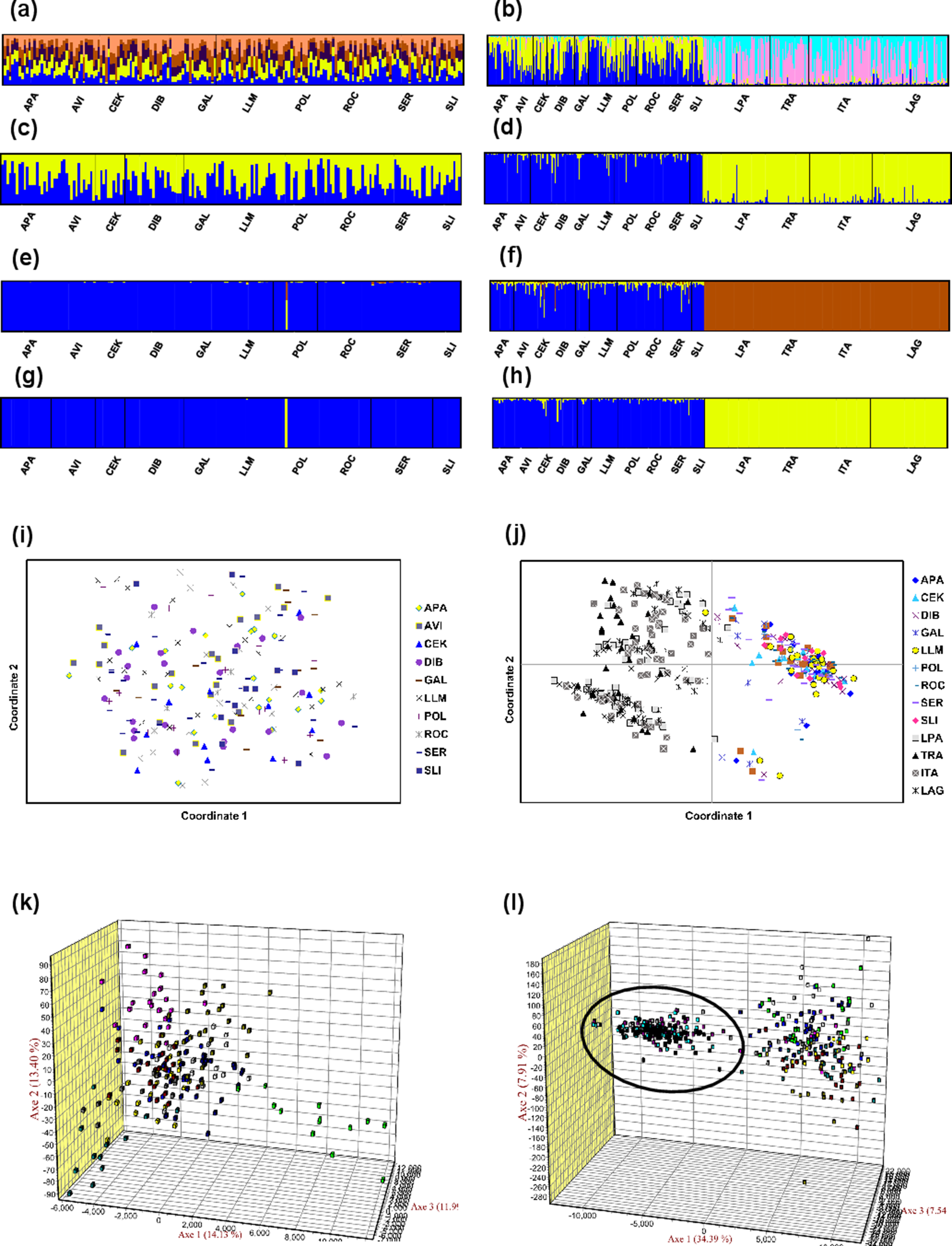
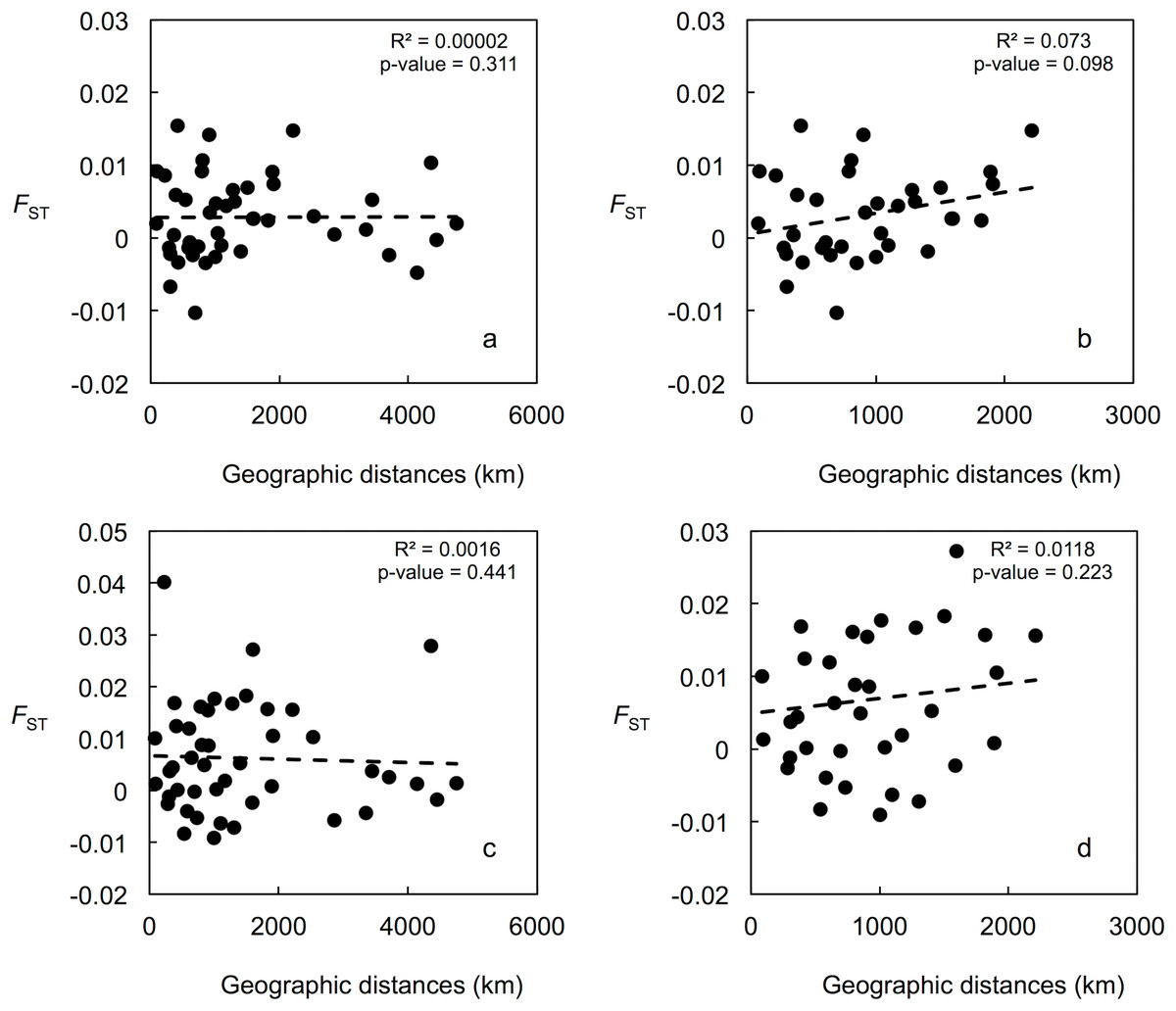
Figure 3: Correlation between population pairwise FST and geographic distance values.
(A) For the 15 putatively neutral loci and all 10 US localities. (B) For the 15 putatively neutral loci and the nine Gulf of Mexico localities. (C) For the US-seven-loci-dataset and all 10 US localities. (D) For the US-seven-loci-dataset and the nine Gulf of Mexico localities.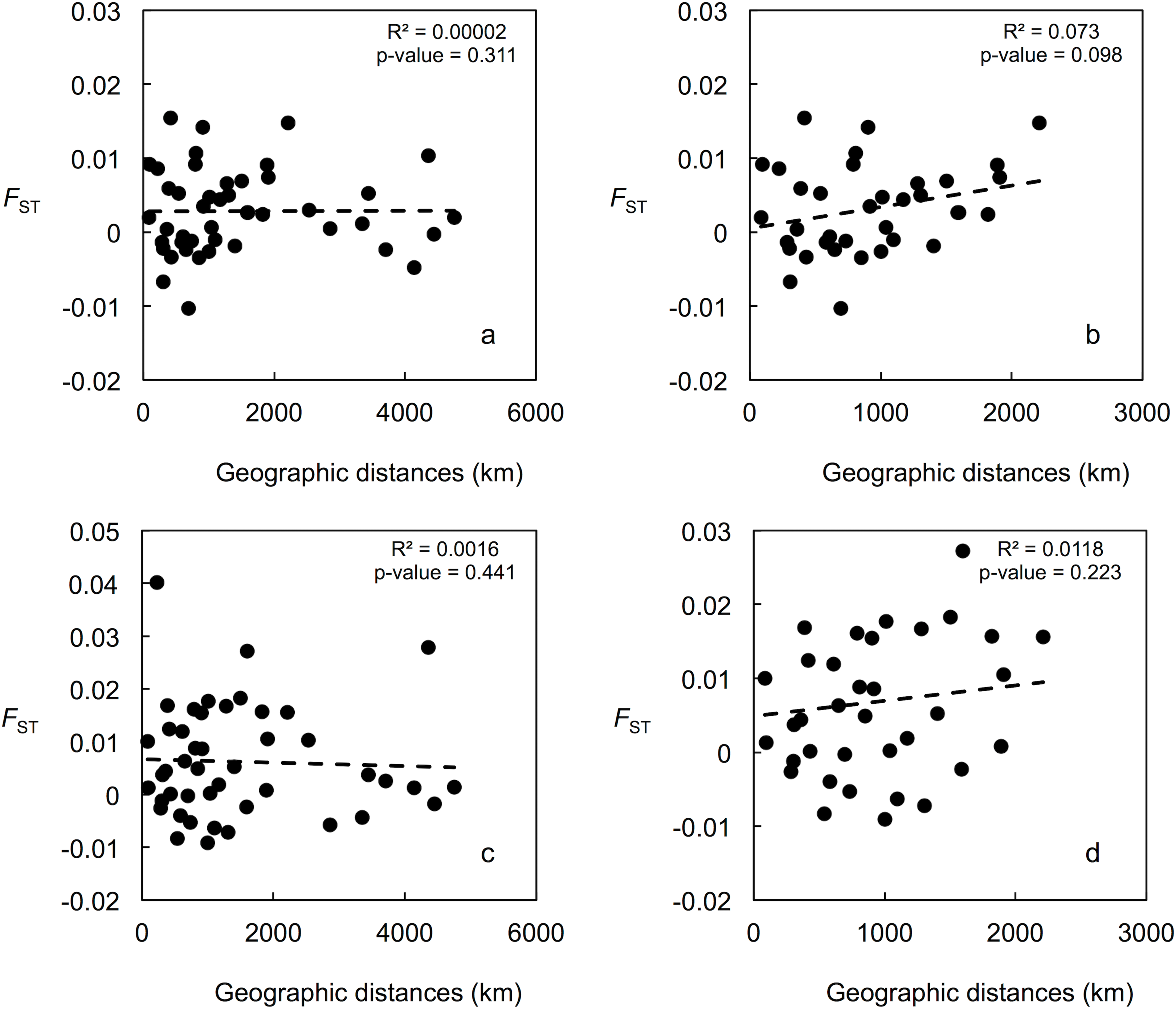
Genetic differentiation between US and Brazilian localities
All FST pairwise comparisons between US and Brazilian localities were high (range 0.11–0.21) and significant (Table S8). AMOVA defining US localities as a group and Brazilian localities as another group found also significant differences between the two regions and this differentiation explains 14.5% of the genetic variation (Table S7). Differences among populations within each group were not significant and accounted for only 0.5% of the variation. The rest of the variation was explained by differences within individuals (44.4%) and among individuals within localities (40.5%). Genetic differentiation between US and Brazil was also clearly observed in STRUCTURE, TESS, PCoA, and FCA analyses (Fig. 2).
Effective population size estimations and demographic tests
The heterozygote excess method estimated values of Ne and 95% CI to be infinite in the US and GOM (Table S9). The LD method estimated infinite or large values for Ne (>2,000), large values for the lower limit of the 95% CI (>1,000), and infinite for the upper limit of the 95% CI. These values can be interpreted as indicative of a very large Ne (Waples & Do, 2010), but see “Discussion.” No signatures of recent bottlenecks were suggested for samples in the US with the Wilcoxon tests using the mutational models TPM (apparently the most appropriate mutational model for microsatellites) and SMM or the Mode-Shift ADT test in the BOTTLENECK program (Table S10). The Wilcoxon test using the mutational model IAM suggested signatures of recent bottlenecks for two US localities.
Analyses of past demographic history using MIGRAINE suggest an expansion of the US blue crab population (Table S11), with estimations of the current population size much larger than estimations of the ancestral effective population size, as indicated by the Nratio (θcur/θanc). The Nratio point estimate obtained for the US-seven-loci dataset using the GSM model (MaxLogLik = −483.3) was 10.27 (95% CI [2.983–19,765]). The Nratio point estimate for the 15 loci dataset under the GSM model (MaxLogLik = −1226.7) was 5.31 (95% CI [2.48–15.44]), whereas under the combined SMM/GSM model (MaxLogLik = –1176.3) this value was 3.05 (95% CI [1.70–5.46]). Relatively precise point estimates were obtained for the different parameters, especially for the 15 loci dataset analyses, as inferred by the clear peaks in the MIGRAINE pairwise likelihood profiles (Fig. 4; see Table S11 for 95% CI). Using a mutation rate of 0.0005, the converted values of N, Nanc and Dg for the analysis of the 15 loci dataset with the SMM/GSM model (which had a better fit for the data) are: N = 17,650 (12,140–32,815) diploid individuals; Dg obtained from Dg/2N = 1,087 (137–6,734) generations; Nanc = 5,785 (3,798–8,400) diploid individuals; Dg obtained from Dgμ = 1,088 (322–2,764) generations.
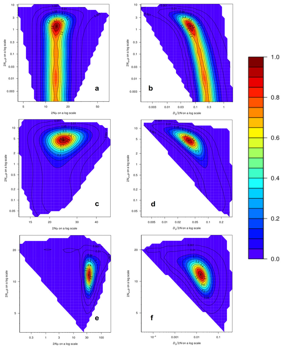
Figure 4: MIGRAINE pairwise likelihood ratio profiles obtained for demographic parameters.
(A and B) The US-seven-loci-dataset with the GSM model. (C and D) The 15 putatively neutral loci with the GSM model. (E and F) The 15 putatively neutral loci with the SMM/GSM model. (A) (C) and (E) Ancestral effective population size 2Nancµ(θanc) vs. current effective population size 2Nµ(θcur). (B) (D) and (F) Ancestral effective population size 2Nancµ(θanc) vs. timing of the demographic history events Dg/2N(D). A very recent expansion is detected for all three models with relatively precise D estimates (see Table S11 for 95% CI). Effective population sizes are also relatively precise and large as shown here (one peak) for all three models (see Table S11 for 95% CI).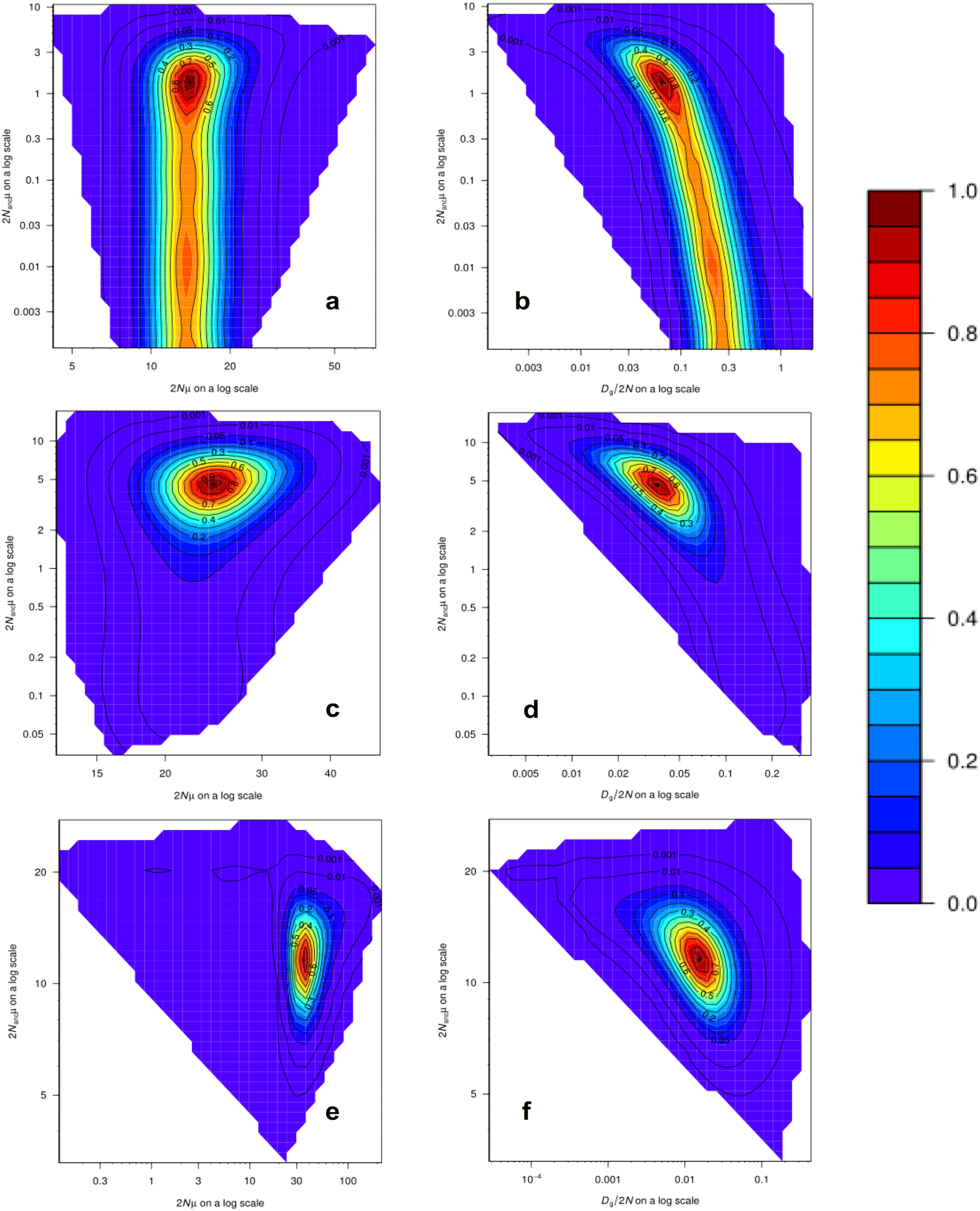
Discussion
This study is the first to investigate microsatellite-based population structure at a large geographic scale for the blue crab within its US range. Prior studies of this species based on a smaller number of microsatellites examined smaller areas restricted to the US Atlantic coast (Cushman & Darden, 2017; Steven et al., 2005). Our results are congruent with previous reports of substantial gene flow, and thus low levels of genetic differentiation in the blue crab among localities in the GOM or throughout its entire US distribution (Berthelemy-Okazaki & Okazaki, 1997; Feng, Williams & Place, 2017; McMillen-Jackson & Bert, 2004; McMillen-Jackson, Bert & Steele, 1994; Yednock & Neigel, 2014b).
Results of genetic differentiation were highly consistent between the dataset that excluded and the dataset that included the loci with high frequency of null alleles and hence deviations of HWP (i.e., the US-seven-loci-dataset and 15-loci-dataset, respectively). Thus, the conclusion of a lack of, or very weak, genetic differentiation for the blue crab in the US seems very robust, even in the presence of loci with null alleles. In the case of FST estimations, this is consistent with the prediction that although failure to correct for the presence of null alleles can lead to overestimation of FST when population differentiation is significant, such FST estimates are regarded as unbiased when population structure is absent (Chapuis & Estoup, 2007), which appears to be the case for the blue crab. FST estimations using the US-seven-loci dataset, which are not expected to be highly affected by null alleles, were very low with and without correcting for null alleles: average pairwise FST was 0.008 and 0.006, respectively. Lower values were obtained for all 15 putatively neutral loci with and without correcting for null alleles: average pairwise FST was 0.006 and 0.003, respectively. None of the uncorrected FST pairwise comparisons were significant using the 15-loci dataset, and only one was significant using the US-seven-loci-dataset, according to the FDR test (FDR ≤ 0.05). After correction for null alleles, the 95% CI of only four comparisons, in both the 15-loci and US-seven-loci datasets (albeit different pairs in each dataset analysis) excluded zero, but their lower interval values were very close to zero, and one was negative. Thus, we interpret that in general, the FST results indicate a lack of, or very weak, genetic differentiation for the blue crab in the US.
Similarly to FST estimations, GST (0.006 and 0.004 for the US-seven-loci-dataset and the 15 putatively neutral loci, respectively), another measure of fixation; and DST (0.004 and 0.002 for the US-seven-loci-dataset and the 15 putatively neutral loci, respectively), which quantifies allelic differentiation; were close to zero. Fixation and allelic differentiation measures quantify complementary aspects of population structure, although they do not necessarily correspond to each other (Jost et al., 2018). Nonetheless, GST approaches zero when the demes are identical in allele composition and frequencies (or when within-deme heterozygosity is high), whereas DST approaches zero if, and only if, all demes are identical (Jost et al., 2018). Thus, we again interpret these results as panmixia, or very weak genetic differentiation, for the blue crab in the US.
Population structure was also not detected using assignment tests (i.e., STRUCTURE and TESS), which have been shown to be highly insensitive to the presence of null alleles (Carlsson, 2008), even in species with a high null allele frequency (Rico et al., 2017). Even though in the STRUCTURE analyses the Evanno method suggests K values between three and nine, and the Puechmaille (2016) estimators suggest K = 2, mean LnP (K) was higher for K = 1 in all analyses, and STRUCTURE plots did not show evidence of any genetic structure within the US. Performance of the Evanno method has been questioned (Janes et al., 2017), whereas the Puechmaille (2016) estimators have not been tested widely, and our results suggest that they may be problematic in the case of panmictic populations. Nonetheless, Latch et al. (2006) conducted simulations of a subdivided population and found that STRUCTURE could not detect more than one population at an FST of 0.01, the lowest value they used. For this reason, we conducted analyses using the STRUCTURE LOCPRIOR setting, which is suggested in cases of weak structure and does not tend to find structure when none is present (see STRUCTURE Manual). These results also suggest that there is no population structure, with r-values much higher than the values interpreted as indicative that locations are informative. AMOVA, DAPC, PCA, FCA, and BayesAss results also did not suggest any genetic structure within the US. IBD also does not appear to be occurring for the blue crab within the US.
Conformance to HWP for pooled data at six loci is also consistent with a large panmictic population in the US. Five of these loci were not suggested to have null alleles, and the remaining one had a low percentage of potential null alleles. Null alleles could have contributed to deviations of HWP in the other loci, as they artificially inflate homozygosity. Similarly, low frequency of private alleles in the populations sampled in our study is also consistent with substantial gene flow. Average pairwise FST using the private alleles method was also very low (0.002 for the US-seven-loci-dataset and 0.005 for the 15 putatively neutral markers), suggesting substantial gene flow.
Remarkably similar values of genetic diversity to those reported in our study were found in a study in Charleston Harbor estuary, South Carolina (Cushman & Darden, 2017), that used six microsatellite loci, of which five overlap with our study. Both studies found very similar average number of alleles (27.8 vs. 28.8, for Charleston Harbor estuary and our study, respectively) and average expected heterozygosity (0.78 vs. 0.774, respectively) for the five loci in common. Null alleles have been shown to have weak effects on expected heterozygosity in species characterized by high prevalence of null alleles (Chapuis et al., 2008). The high similarity in genetic diversity between two independent studies is consistent with the finding of substantial gene flow across the US, suggesting that a subsample from a very small area (i.e., Charleston Harbor estuary) adequately captures the genetic diversity found in the whole region.
The South Carolina study (Cushman & Darden, 2017) reports a null allele frequency of 0 for CSA-121, 0.004 for CSA-035, 0.012 for CSA-073, 0.059 for CSC-007 (this is the only marker they found deviating from HWE), and 0.093 for CSC-094. Pooling data across localities in our study, MICRO-CHECKER suggests a frequency of null alleles of 0.005 for CSA-121, 0.127 for CSA-035, 0.041 for CSA-073, 0.077 for CSC-007 and 0.037 for CSC-094. Differences in the sampled range could have contributed to the observed differences between the two studies. In addition, the South Carolina study used CERVUS 3.0 (Kalinowski, Taper & Marshall, 2007) to detect null alleles, and it is reported that different methods to detect null alleles can provide different results (Dabrowski et al., 2015). Differences for CSA-035, however, are very marked. Although both studies observed 47 alleles for this locus, the South Carolina study reports an allelic size range of 148–256, whereas we found a range of 160–258. We sought to examine the South Carolina dataset, but unfortunately the authors of Cushman & Darden (2017) did not make it available, despite our request. Null alleles have also been reported for the southern Brazilian populations study (Lacerda et al., 2016), which used the same five loci we had in common with the South Carolina study. Null alleles are likely to occur in populations with large effective population sizes (Chapuis & Estoup, 2007), which appears to be the case for the blue crab according to our results.
Including all 16 loci, the average number of alleles per locus and expected heterozygosity for the blue crab in our study is 18.12 and 0.74, respectively. When the five microsatellites with di-motifs in our study are excluded, average number of alleles and expected heterozygosity dropped to 9.36 and is 0.64, respectively. Genetic diversity in the US was higher than in southern Brazil for the seven loci in common (three di-, four tetra-motif) between both datasets, with an average number of alleles per locus (26 vs. 28.14) and expected heterozygosity (0.58 vs. 0.82) for southern Brazil and US, respectively. Genetic diversity estimations for the blue crab in the US are also higher than those reported for the brown swimming crab C. bellicosus along the coast of Sonora, Gulf of California, Mexico. For this species, average number of alleles per locus, average effective number of alleles per locus, and mean observed and expected heterozygosity were 6.08, 3.9, 0.49, and 0.50, respectively (Cisneros-Mata et al., 2019).
High genetic diversity for the blue crab in the US has been also reported for mitochondrial markers (Feng, Williams & Place, 2017; McMillen-Jackson & Bert, 2004), which is in general much higher than that reported for other invertebrates, and at the upper end of other crustaceans (Feng, Williams & Place, 2017). In the GOM, Darden (2004) found 146 unique haplotypes (n = 213) of C. sapidus with 216 variable sites for a 622-bp COI fragment. For comparison, a study of C. bellicosus along most of its distribution in the Gulf of California and Pacific Baja California reports only 23 haplotypes (n = 67) with 26 variable sites for a 658-bp COI fragment (Pfeiler et al., 2005). Nonetheless, the high estimated mtDNA diversity for C. sapidus may be influenced by the occurrence of high levels of heteroplasmy in this species (Williams, Feng & Place, 2017). MtDNA diversity estimates could also be inflated by misidentification; a highly divergent COI sequence found by Feng, Williams & Place (2017) could belong to C. similis or to a highly divergent lineage of C. sapidus so far restricted to Brazil (Rodrigues et al., 2017). Unfortunately, this cannot be verified because neither of these studies has made its sequence data publicly available. High genetic diversity has been also reported in DNA sequences from four nuclear markers of the blue crab in Louisiana (Yednock & Neigel, 2014a). Thus, different genetic markers indicate that the blue crab harbors high levels of genetic diversity along its US range.
Inbreeding does not appear to be a problem for blue crabs in the US. Low inbreeding was estimated for individual loci in the US-seven-loci-dataset (average GIS = 0.02). Null alleles, which can inflate inbreeding estimations, are not expected to largely bias inbreeding estimations for these loci, because they were absent, or in low frequency. A low average inbreeding value was also obtained for these loci when considered a single panmictic population (0.015). Similarly, unbiased estimations of the inbreeding coefficient for all 15 putatively neutral loci using INEST resulted in a value of 0 for the “null alleles and genotyping failures” (nb) model, and 0.021 for the “null alleles, inbreeding and genotyping failures” (nfb) model. Low mean relatedness values within localities (average = −0.0023) are consistent with low inbreeding and high gene flow. In the South Carolina study, estimated FIS values are low (average = 0.06), which is similar to the value estimated in southern Brazil (0.056). Similarly, low FIS values were reported in the Louisiana coast (Yednock & Neigel, 2014a). Therefore, our results and those of other studies suggest low levels of inbreeding for the blue crab in the US.
Even though our sampling did not aim to compare temporal changes within localities, the lack of genetic differentiation among different localities sampled at different times (our samples from Lower Laguna Madre and Chesapeake Bay were collected in 2015, while all others in 2014) implies temporal genetic stability. Similarly, the samples in Cushman & Darden (2017), from Charleston Harbor estuary, South Carolina, were collected in 2012 and 2013, and the number of alleles and expected heterozygosity for both years are very similar to our values. Thus, temporal genetic stability appears to occur at a large scale. Other studies, however, have reported temporal genetic differences, but they generally occurred at a single locality and may have resulted from extraordinary events that affected the genetic makeup in localized areas. Yednock & Neigel (2014a) sampled blue crabs from nine localities in the Louisiana coast in 2010, four of which were sampled again in 2011. They did not find evidence of significant geographic or temporal genetic differentiation, with the exception of one locality that showed significant allelic frequency shifts between the 2 years for the four nuclear loci they examined. They speculate that events related to the 2010 Deepwater Horizon Oil Spill may have contributed to these differences in this locality. The other localities, however, did not show allelic changes, despite also being in the coastal area affected by the oil spill (one was separated by just ~26 Km from the one that showed temporal differences). Similarly, Feng, Williams & Place (2017) found temporal genetic differences in samples collected during 5 years in the same locality in Rhode River, Chesapeake Bay. A sample collected in 2003 was different to samples collected in 2004, 2005, 2006, and 2007, which could not be distinguished from each other. They suggest that abnormal water circulation patterns and hurricane Isabel, both of which occurred in 2003, could have altered larval dispersal and juvenile recruitment.
Two previous studies are at odds with the findings of high levels of gene flow for the blue crab in the US. On the basis of three moderately polymorphic allozymes, Kordos & Burton (1993) report significant spatial and temporal population genetic differences in megalopa and adult samples in the Texas coast. Nonetheless, the use of only three informative allozyme markers, of which one or more could be under selection due to their protein-coding nature, limits the robustness of inferred patterns (Karl & Avise, 1992). Supporting this notion, another allozyme study (McMillen-Jackson, Bert & Steele, 1994), inferred levels of gene flow consistent with panmixia among blue crab populations from New York to Texas. Although these authors observed genetic patchiness on local and range-wide geographic scales, and one locus also exhibited temporal variation, they suggest that differences in pre-settlement larval patches and subsequent selection at settlement may contribute to these patterns in the presence of high gene flow. Furthermore, the genetic differences among megalopa populations detected by Kordos & Burton (1993) could be due to misidentifications, as the morphological characters they used to distinguish C. sapidus from C. similis were later deemed unreliable by Sullivan & Neigel (2017). Indeed, Sullivan & Neigel (2017) found a temporal composition shift in the abundance of C. similis and C. sapidus megalopae that parallels changes in the allozyme allele frequencies reported for blue crab megalopae at the same localities studied by Kordos & Burton (1993). Genetic differences between concurrent samples of megalopae (n = 32 individuals) and adults (n = 49) at a locality in Chesapeake Bay have also been reported by Feng, Williams & Place (2017) at two (out of four microsatellite loci). Nonetheless, these inferences could be biased by the large number of alleles per locus (49–54), compared to the examined sample sizes.
The second study that reported significant population structure for the blue crab within the US, examined mitochondrial COI sequences and found differences between the eastern and western GOM, and among some localities within the western GOM (Darden, 2004). Based on these results, the Gulf States Marine Fisheries Commission proposed two blue crab stocks for management within the US GOM, with their division around Apalachicola, Florida (reviewed in Perry & VanderKooy, 2015). The use of mitochondrial markers to infer population connectivity and genetic diversity in the blue crab, however, appears problematic due to extremely high levels of mtDNA heteroplasmy detected in this crustacean (Williams, Feng & Place, 2017). Cloning and sequencing of segments of the ND2, ND4, and COI mitochondrial loci detected as many as 24 haplotypes in a single individual and the dominant haplotype accounted for as little as 43.9% of the total sequences (Williams, Feng & Place, 2017). This may explain the extremely high mitochondrial genetic diversity observed in this crab. Our study, which included populations at both sides of this proposed division, as well as previous studies in the region (one of which also used a mitochondrial marker), did not find evidence of genetic structure within the US GOM. Yednock & Neigel (2014a), based on nuclear protein-coding genes sequences, found no population genetic differences between samples collected in Louisiana and one sample collected in the Lower Laguna Madre, Texas.
The picture emerging from independent studies using different types of markers is that the blue crab experiences high levels of gene flow in the US Atlantic and GOM region, likely corresponding to a very large panmictic population. This is remarkable considering the variation in environmental factors (e.g., salinity, temperature), potential barriers for dispersal, and genetic breaks observed for other marine species in this region, which include differentiation between the Atlantic and GOM, the East and West GOM, and differentiation between the Laguna Madre and other GOM localities (Milá et al., 2017; Neigel, 2009). A recent study (Plough, 2017) that used >9,600 single nucleotide polymorphisms (SNPs) obtained with RAD-sequencing, however, reports low but significant genetic differentiation (FST = 0.0103) between blue crabs collected in Panama City, Florida (GOM), and Agawam River, Massachusetts, at the northern US Atlantic (only these two US populations were included in that study). Thus, it is possible that the use of high-throughput sequencing methods could reveal low levels of genetic differentiation that may be present for this species in the US.
High levels of gene flow have also been determined for the blue crab along 740 km in southern Brazil (Lacerda et al., 2016). Despite the apparent extraordinary long distance dispersal potential of this species, there are limits to genetic homogenization across the blue crab distribution. Yednock & Neigel (2014a) report strong genetic differentiation between samples in the GOM (from Louisiana and Texas) and Venezuela. We also found strong genetic differentiation between our US samples and those from Lacerda et al. (2016) in southern Brazil. We acknowledge, however, that combining microsatellite data from different labs can be problematic (Morin et al., 2009). Nonetheless, a strong indication of genetic differentiation between the two regions that may be largely insensitive to potential bias from the combination of data from the two labs is the observation of marked differences in expected heterozygosity in six of the seven microsatellites between the US and southern Brazil. Expected heterozygosity for southern Brazil and the US is 0.59 and 0.84, respectively. This finding is congruent with the results of Rodrigues et al. (2017), which examined COI DNA sequences and reported significant differences between the two regions; although as mentioned previously, this marker is problematic for genetic structure studies because of high levels of mitochondrial heteroplasmy in this species. Similarly, the RAD-sequencing study of Plough (2017) found that two individuals from Porto Alegre, Brazil, within the region sampled by Lacerda et al. (2016), are highly differentiated from those in the two US localities he examined. A disjunct distribution for the blue crab has been suggested (Rodrigues et al., 2017; Santos & D’Incao, 2004), with a gap in northern South America (i.e., from Guyana to northern Brazil), although this needs to be verified. Future sampling efforts are needed between the US and southern Brazil to understand the limits of the populations these two regions harbor, whether other differentiated populations are present across the blue crab range, and what factors may be associated with genetic differentiation.
Estimations of Ne suggest a very large effective population size for the blue crab in the US, which is congruent with the extremely large population size inferred from the thousands of tons that are harvested each year for this species in this region. It has been suggested that precise Ne estimates using the LD method can be obtained with this method for relatively small populations (Ne < 200), and small populations are not likely to be mistaken for large ones; but it is very difficult to obtain reliable estimates for large populations with this method (Waples & Do, 2010). Estimations of Ne in the Charleston Harbor estuary using the LD method also suggest a very large population (Cushman & Darden, 2017). They obtained negative values for Ne estimations, which are interpreted as indicative of a very large Ne, with lower 95% CI values ranging from 334–4,267. However, the interpretation of negative values using the LD method as indicating very large (infinite) Ne has been challenged. A recent study indicates that for medium-sized populations (one million individuals) and common sample sizes (50 individuals), negative estimates with the LD method are likely to occur, and that on average Ne estimates are negatively biased (Marandel et al., 2019). Through simulations, they found that to obtain sufficiently precise estimates of Ne, ~ 1% of the total number of individuals in a population might need to be sampled. This probably corresponds to millions of individuals in the case of the blue crab US population.
Our demographic analyses suggest a recent expansion of the US blue crab population. According to the analysis of the 15 loci dataset with the SMM/GSM model, which had the best fit for the data, the population grew between 1.7 and 5.5 times. Using a mutation rate of 5 × 10⁻⁴, a large Ne was estimated (17,650 individuals), which is consistent with the previous analyses of Ne. The expansion appears to have occurred recently, based on the point estimate for Dg (i.e., the time of the demographic change in generations) of 1,088 generations ago, and given that blue crabs live between 2 and 3 years. Considering the upper 95% CI value of Dg (6,734 generations), which was obtained from Dg/2N, this expansion could have occurred several thousands years ago. Although mutation rates can be very variable, changes in one order of magnitude still result in large Ne and a recent time of demographic change estimations. Assuming mutation rates of 5 × 10⁻³ and 5 × 10⁻⁵, conversions of Ne result in 1,765 and 176,500 individuals, respectively, and of Dg in 108.7 and 10,880 generations, respectively. The demographic expansion of the blue crab probably occurred after the end of the last glacial period (11,650 years ago), during the Holocene, when the seas became warmer. Several marine and coastal taxa also exhibit signatures consistent with range expansions since the Last Glacial Maximum (Eberl et al., 2013; Hurtado, Lee & Mateos, 2013; Jenkins, Castilho & Stevens, 2018; Marko et al., 2010). The lineage of C. sapidus is estimated to have diverged from its sister lineage C. toxotes 0.6 to 6.4 Mya (Robles et al., 2007). Fossils of Callinectes crabs in the US Atlantic coast have been reported from the Pleistocene and Miocene (Rathbun, 1935).
Conclusion and future directions
Our population genetics analyses based on microsatellites indicate substantial gene flow, high genetic diversity, a large effective population size, and no indication of inbreeding or recent bottlenecks for the blue crab in its US distribution. Lack of genetic structure in the US is consistent with other studies using different types of markers that also suggest a panmictic population in this region, with rare instances of some local temporal genetic differentiation. Detection of population structure in marine organisms characterized by extremely large populations and high dispersal potential, and/or with recently diverged populations, however, may be difficult using neutral markers, and the use of non-neutral markers has been recommended (Allendorf, Hohenlohe & Luikart, 2010; Andre et al., 2011; Liu, Sun & Hurtado, 2013; Russello et al., 2012). Therefore, it is important to use genomic techniques, such as RAD-sequencing or whole genome sequencing, to study population genetic differentiation in the blue crab, which should allow identification of potential non-neutral markers. The blue crab genome is highly variable, as indicated by the hundreds of thousands of SNPs identified in a transcriptome of this species (Yednock, Sullivan & Neigel, 2015). It is also important to include samples between the US and southern Brazil, to better understand the limits of the populations these two regions harbor, and establish whether other differentiated populations are present across the blue crab range.