The Bayesian confidence intervals for measuring the difference between dispersions of rainfall in Thailand

Noppadon Yosboonruang; Sa-Aat Niwitpong; Suparat Niwitpong

doi:10.7717/peerj.9662

The Bayesian confidence intervals for measuring the difference between dispersions of rainfall in Thailand

Noppadon Yosboonruang, Sa-Aat Niwitpong, Suparat Niwitpong

Department of Applied Statistics, Faculty of Applied Science, King Mongkut’s University of Technology North Bangkok, Bangkok, Thailand

DOI: 10.7717/peerj.9662

Published: 2020-08-06
Accepted: 2020-07-15
Received: 2020-04-13

Academic Editor: Matthew Wilson

Subject Areas: Statistics, Computational Science, Natural Resource Management, Ecohydrology, Environmental Contamination and Remediation
Keywords: Coefficient of variation, Fiducial generalized confidence interval, The left-invariant Jeffreys prior, Jeffreys’ Rule prior, Bootstrap method, Uniform prior

Copyright: © 2020 Yosboonruang et al.
Licence: This is an open access article distributed under the terms of the Creative Commons Attribution License, which permits unrestricted use, distribution, reproduction and adaptation in any medium and for any purpose provided that it is properly attributed. For attribution, the original author(s), title, publication source (PeerJ) and either DOI or URL of the article must be cited.

Cite this article: Yosboonruang N, Niwitpong S, Niwitpong S. 2020. The Bayesian confidence intervals for measuring the difference between dispersions of rainfall in Thailand. PeerJ 8:e9662 https://doi.org/10.7717/peerj.9662

The authors have chosen to make the review history of this article public.

Abstract

The coefficient of variation is often used to illustrate the variability of precipitation. Moreover, the difference of two independent coefficients of variation can describe the dissimilarity of rainfall from two areas or times. Several researches reported that the rainfall data has a delta-lognormal distribution. To estimate the dynamics of precipitation, confidence interval construction is another method of effectively statistical inference for the rainfall data. In this study, we propose confidence intervals for the difference of two independent coefficients of variation for two delta-lognormal distributions using the concept that include the fiducial generalized confidence interval, the Bayesian methods, and the standard bootstrap. The performance of the proposed methods was gauged in terms of the coverage probabilities and the expected lengths via Monte Carlo simulations. Simulation studies shown that the highest posterior density Bayesian using the Jeffreys’ Rule prior outperformed other methods in virtually cases except for the cases of large variance, for which the standard bootstrap was the best. The rainfall series from Songkhla, Thailand are used to illustrate the proposed confidence intervals.

Introduction

Recently, the Earth’s climate has been changing significantly due to the greenhouse effect, which is causing both rising temperatures and variability in precipitation (Attavanich, 2013). In particular, Thailand, which is an agricultural country, is greatly affected by such phenomena since agriculture mainly relies on rainfall. The amount of rainfall in Thailand fluctuates quite widely due to the influence of the southwest and northeast monsoons (Eso, Kuning & Chuai-Aree, 2015). In previous years, several areas in Thailand have been affected by heavy rain that produced flooding, a major cause of economic, life, and property loss.

It is important to investigate the coefficient of variation of rainfall data series to understand the dynamics of precipitation in each area. Furthermore, the difference between two areas or time periods of heavy rainfall measured with their coefficients of variation is of interest. The government can use this information for advanced planning to prevent problems caused by excessive rainfall. Many researchers have found that rainfall data series follow a bivariate lognormal distribution (a delta-lognormal distribution) (Fukuchi, 1988; Shimizu, 1993; Kong et al., 2012; Maneerat, Niwitpong & Niwitpong, 2019a, 2019b; Yosboonruang, Niwitpong & Niwitpong, 2019b; Yue, 2000).

Confidence interval construction is another method of effective statistical inference for applying to delta-lognormal distributions and methods to construct them have been reported by several researchers. Zhou & Tu (2000) proposed confidence intervals for the mean including a percentile-t bootstrap interval based on sufficient statistics, a bias-corrected maximum likelihood method, and an interval based on a likelihood ratio testing method; the bootstrap interval performed the best for both one-sided and two-sided intervals with a small sample size. Tian (2005) compared the generalized variables method and the generalized pivotal quantity (GPQ) to construct confidence intervals for the mean, between which the generalized variables method was preferable. Tian & Wu (2006) recommended using the adjusted signed log-likelihood ratio statistic to construct confidence intervals for the mean. Chen & Zhou (2006) considered interval estimations for the ratio of or difference between two means using a true generalized pivotal (GP) method, an approximate GP method, a signed log-likelihood ratio method, and a modified signed log-likelihood ratio method; their results show that the approximate GP method performed the best. Fletcher (2008) used three methods, Aitchison’s estimator, a modification of Cox’s method, and a profile-likelihood interval, to construct confidence intervals for the mean; they found that the profile-likelihood interval was the best unless the sample size was small with a low-to-moderate level of skewness. Li, Zhou & Tian (2013) presented an approximate GPQ and the fiducial quantity to establish confidence intervals for the mean; their results indicate that the fiducial method was the most suitable. Wu & Hsieh (2014) introduced the generalized confidence interval (GCI) to construct confidence intervals for the mean that were better than Aitchison’s method, a modified Land’s method, and the profile-likelihood interval. Maneerat, Niwitpong & Niwitpong (2018) constructed confidence intervals for the mean using GCI, the method of variance estimate recovery (MOVER) based on the variance stabilizing transformation (VST), Wilson’s score, and Jeffrey’s method; GCI and the three MOVER methods had similar performances except for cases where the probability had values close to zero and the coefficient of variation was large. Moreover, they compared GCI and MOVER based on a weighted beta distribution and VST to construct confidence intervals for the mean and recommended MOVER based on VST (Maneerat, Niwitpong & Niwitpong, 2019b). In addition, Maneerat, Niwitpong & Niwitpong (2019a) suggested Bayesian methods to construct the highest posterior density (HPD) intervals for a single mean and the difference between two means.

Apart from the mean, the coefficient of variation, which is defined as the ratio of the standard deviation to the mean, has been used to solve this statistical problem. There have been many studies focused on confidence interval estimation for the coefficient of variation of normal and non-normal distributions. For instance, Wong & Wu (2002) constructed confidence intervals by developing small sample asymptotic methods for both normal and non-normal models. In addition, confidence interval estimations for the coefficient of variation of a normal distribution have been reported by Tian (2005), Donner & Zou (2012), and Wongkhao, Niwitpong & Niwitpong (2015). Confidence intervals for the coefficient of variation have been established for skewed distributions. Sangnawakij & Niwitpong (2017a) presented confidence interval estimations for the coefficient of variation and the difference between coefficients of variation based on MOVER, GCI, and asymptotic confidence interval for two-parameter exponential distributions, their results indicating that GCI outperformed the other methods. Thangjai & Niwitpong (2017) proposed confidence intervals for the weighted coefficients of variation of two-parameter exponential distributions using the adjusted MOVER, GCI, and large sample methods, their result showing that GCI was the best choice. Yosboonruang, Niwitpong & Niwitpong (2018) constructed confidence intervals for the coefficient of variation of a delta-lognormal distribution using GCI and a modified Fletcher method and found that GCI was the most appropriate. Yosboonruang, Niwitpong & Niwitpong (2019a) presented the fiducial generalized confidence interval (FGCI) and MOVER to construct confidence intervals for three parameters of a delta-lognormal coefficient of variation. They reported that FGCI was suitable for small sample sizes while MOVER performed similarly well to FGCI when the sample sizes were large. In addition, they constructed confidence intervals using Bayesian methods with equitailed confidence intervals and the HPD interval and compared them with FGCI; their results show that the Bayesian equitailed confidence interval was appropriate in all cases (Yosboonruang, Niwitpong & Niwitpong, 2019b).

Confidence interval estimations for functions of the coefficient of variation are of interest. For normal distributions, Donner & Zou (2012) presented MOVER to construct a confidence interval for the difference between two coefficients of variation. Their proposed method performed well for both the coverage percentage and balance between the tail errors. Niwitpong (2015) proposed confidence intervals for the difference between the coefficients of variation with bounded parameters; their results show that their proposed confidence intervals outperformed other classical ones in terms of the coverage probability and the average length.

For skewed distributions, Buntao & Niwitpong (2012) constructed confidence intervals for the difference between coefficients of variation for lognormal and delta-lognormal distributions by using the GP method and a closed-form method of variance estimation; their results for both lognormal and delta-lognormal distributions indicate that the GP method was better than the closed-form method in all cases. Buntao & Niwitpong (2013) produced confidence intervals for the ratio of the coefficients of variation of delta-lognormal distributions based on the GP method and the MOVER based Wald interval; they suggested that the GP method was the most appropriate. Sangnawakij & Niwitpong (2017b) constructed new confidence intervals for functions of the difference between and the ratio of the coefficients of variation with restricted parameters in two gamma distributions; they found that the expected lengths of the proposed confidence intervals were shorter than other classical estimators.

Although a number of previous studies have reported on constructing confidence intervals for several parameters in each distribution, there has been only one study on constructing confidence intervals for the difference between the coefficients of variation of two delta-lognormal distributions. Constructing confidence intervals using general methods are quite complex. Furthermore, results have revealed that the performances of these methods are not consistent since the coverage probabilities are less than the target in a few cases. From the perspective of rainfall data, estimating the difference between two independent coefficients of variation can help to elucidate rainfall variability in terms of time or area. It is useful for forecasting rainfall to help in planning for and managing risky situations that can arise from rainfall variation.

In this study, the difference between the coefficients of variation of two delta-lognormal distributions was investigated. In previous studies (Donner & Zou, 2012; Li, Zhou & Tian, 2013; Wu & Hsieh, 2014; Sangnawakij & Niwitpong, 2017a; Thangjai & Niwitpong, 2017; Maneerat, Niwitpong & Niwitpong, 2018, 2019a; Yosboonruang, Niwitpong & Niwitpong, 2018, 2019a), confidence intervals for the difference between the coefficients of variation of two delta-lognormal distributions were constructed using three methods (GCI, FGCI, and MOVER). Our preliminary study indicates that these methods performed similarly, although FGCI is the best due to having the shortest expected length. Therefore, we constructed new confidence intervals for the difference between the coefficients of variation of two delta-lognormal distributions using Bayesian methods and a standard bootstrap (SB) method and compared them with FGCI. The details of each method are presented in the next section, after which the results are presented. Next, the efficacies of the proposed methods for constructing confidence intervals are illustrated using rainfall data in an empirical example, followed by a discussion and conclusions of the study outcomes.

Materials and Methods

In statistical inference and its applications, data containing non-negative values can be skewed and many zero observations can be observed. Aitchison (1955) introduced the delta-lognormal distribution for data series containing non-negative values and true-zero values of the variables. The positive observed values, denoted by n_i(1), have a lognormal distribution, and the true-zero observed values, denoted by n_i(0), have a binomial distribution with the probability of zero observations ${\tilde{δ}}_{i} = 1 - δ_{i}$ , where n_i = n_i(1) + n_i(0). Let X_ij = (X_i1, X_i2, …, X_in_{_i}) be a non-negative random sample from a delta-lognormal distribution with parameters δ_i, μ_i and $σ_{i}^{2}$ , denoted by $X_{i j} \sim Δ (δ_{i}, μ_{i}, σ_{i}^{2})$ . The distribution function of the delta-lognormal distribution presented by Tian & Wu (2006) is (1) $F (x_{i j}; δ_{i}, μ_{i}, σ_{i}^{2}) = (\begin{matrix} {\tilde{δ}}_{i} & ; x_{i j} = 0 \\ {\tilde{δ}}_{i} + δ_{i} H (x_{i j}; μ_{i}, σ_{i}^{2}) & ; x_{i j} > 0, \end{matrix}$ where $H (x_{i j}; μ_{i}, σ_{i}^{2})$ is the lognormal cumulative distribution function. Assume that Y_ij = ln(X_ij), i = 1, 2, j = 1, 2,…,n_i(1) is a normal distribution with mean μ_i and variance $σ_{i}^{2}$ . Thus, the population mean and variance of a delta-lognormal distribution as presented by Aitchison (1955) are $E (X_{i j}) = δ_{i} \exp (μ_{i} + σ_{i}^{2} / 2)$ and $V a r (X_{i j}) = δ_{i} \exp (2 μ_{i} + σ_{i}^{2}) [\exp (σ_{i}^{2}) - δ_{i}]$ , respectively. Herein, we focus on confidence interval estimations for the difference between the coefficients of variation of two delta-lognormal distributions. The coefficient of variation of a delta-lognormal distribution can be expressed as (2) $C V (X_{i j}) = η_{i} = \frac{\sqrt{V a r (X_{i j})}}{E (X_{i j})} = {[\frac{\exp (σ_{i}^{2}) - δ_{i}}{δ_{i}}]}^{\frac{1}{2}} .$

It is easy to find the difference between two independent coefficients of variation: (3) $γ = η_{1} - η_{2} = {[\frac{\exp (σ_{1}^{2}) - δ_{1}}{δ_{1}}]}^{\frac{1}{2}} - {[\frac{\exp (σ_{2}^{2}) - δ_{2}}{δ_{2}}]}^{\frac{1}{2}} .$

The fiducial generalized confidence interval

The basic concept of the fiducial distribution was introduced by Fisher (1930). Moreover, statistical inference using fiduciality can be found in several studies (Dawid & Stone, 1982; Aldrich, 2000; Hannig et al., 2006; Hannig, Iyer & Patterson, 2006; Hannig, 2009; Hannig & Lee, 2009). After that, Li, Zhou & Tian (2013) proposed the generalized fiducial quantity (GFQ) of a population mean by using the concept of fiducial inference and then constructed confidence intervals for the mean based on the fiducial of a lognormal distribution with excess zeros. Furthermore, Yosboonruang, Niwitpong & Niwitpong (2019a) recommended FGCI to construct confidence intervals for the coefficient of variation of a delta-lognormal distribution. From Hannig (2009) and Li, Zhou & Tian (2013), the GFQs for δ_i and $σ_{i}^{2}$ are (4) $T_{δ_{i}} \sim \frac{1}{2} B e t a (n_{i (1)}, n_{i (0)} + 1) + \frac{1}{2} B e t a (n_{i (1)} + 1, n_{i (0)})$ and (5) $T_{σ_{i}^{2}} = \frac{(n_{i (1)} - 1) {\hat{σ}}_{i}^{2}}{U_{i}},$ respectively, where $U_{i} \sim χ_{n_{i (1)} - 1}^{2}$ . Next, the GFQ for γ can be defined as (6) $T_{γ} = T_{η_{1}} - T_{η_{2}} = {[\frac{\exp (T_{σ_{1}^{2}}) - T_{δ_{1}}}{T_{δ_{1}}}]}^{\frac{1}{2}} - {[\frac{\exp (T_{σ_{2}^{2}}) - T_{δ_{2}}}{T_{δ_{2}}}]}^{\frac{1}{2}} .$

Therefore, the 100 (1 − α)% confidence interval for γ is (7) $C I_{γ}^{F G C I} = [T_{γ, (l)}, T_{γ, (u)}] = [T_{γ} (α / 2), T_{γ} (1 - α / 2)],$ where T_γ (α/2) and T_γ (1 − α/2) are the 100 (α/2)-th and 100 (1 − α/2)-th percentiles of the distribution of T_γ, respectively.

The algorithm to construct FGCI

Generate datasets x_ij, i = 1,2, j = 1,2,…,n_i from the delta-lognormal distribution.
Generate $B e t a (n_{i (1)}, n_{i (0)} + 1)$ and $B e t a (n_{i (1)} + 1, n_{i (0)})$ .
Compute T_{δ_i}, $T_{σ_{i}^{2}}$ , and T_γ.
Repeat steps 2 and 3 5,000 times.
Compute the $100 (1 - α) %$ confidence intervals for γ.
Repeat steps 1–5 15,000 times.

Bayesian methods

A delta-lognormal distribution is a combination of the two distributions mentioned earlier, with unknown parameters comprising δ_i, μ_i and $σ_{i}^{2}$ , denoted as $θ = (δ_{i}, μ_{i}, σ_{i}^{2})$ . To compare the two population coefficients of variation, the joint likelihood function is expressed as (8) $L (θ | x_{i j}) \propto \prod_{i = 1}^{2} {{\tilde{δ}}_{i}^{n_{i (0)}} δ_{i}^{n_{i (1)}} \prod_{j = 1}^{n_{i (1)}} \frac{1}{σ_{i}} \exp [- \frac{1}{2 σ_{i}^{2}} {(\ln x_{i j} - μ_{i})}^{2}]} .$

Our approach points toward the difference between two independent coefficients of variation, given as Eq. (3), thus the unknown parameters are δ_i, μ_i and $σ_{i}^{2}$ , denoted as $\tilde{θ} = (δ_{1}, μ_{1}, σ_{1}^{2}, δ_{2}, μ_{2}, σ_{2}^{2})$ . The Fisher information of $\tilde{θ}$ computed by the second-order derivative of the log-likelihood function which is defined as (9) $I (\tilde{θ}) = - E (\frac{\partial^{2} \ln L}{\partial {\tilde{θ}}^{2}}) .$

By Eq. (8), the Fisher information matrix for $\tilde{θ}$ becomes (10) $I (\tilde{θ}) = d i a g [\begin{matrix} \frac{n_{1}}{{\tilde{δ}}_{1} δ_{1}} & \frac{n_{1} δ_{1}}{σ_{1}^{2}} & \frac{n_{1} δ_{1}}{2 {(σ_{1}^{2})}^{2}} & \frac{n_{2}}{{\tilde{δ}}_{2} δ_{2}} & \frac{n_{2} δ_{2}}{σ_{2}^{2}} & \frac{n_{2} δ_{2}}{2 {(σ_{2}^{2})}^{2}} \end{matrix}] .$

To establish confidence intervals using the Bayesian methods, the left-invariant Jeffreys, the Jeffreys’ Rule, and uniform priors were used. In this study, we are interested in constructing the HPD intervals. The probability of the shortest interval is discovered when the posterior density value at the lower and upper limits is equal, thus the upper and lower tail areas are not necessarily equal (Bolstad & Curran, 2017).

The Bayesian method using the left-invariant Jeffreys prior

Rainfall series that consist of zero and non-zero values follow a combination of two distributions: binomial and lognormal. As mentioned previously, the parameter of interest for a binomial distribution is ${\tilde{δ}}_{i}$ and by using the Fisher information matrix of ${\tilde{δ}}_{i}$ , we can obtain the invariant Jeffreys prior by the square root of the determinant of Fisher information matrix which is defined as (11) $p ({\tilde{δ}}_{i}) \propto \sqrt{| I ({\tilde{δ}}_{i}) |} \propto {\tilde{δ}}_{i}^{- \frac{1}{2}} δ_{i}^{- \frac{1}{2}},$ which is Beta (1/2,1/2). Subsequently, the posterior distribution of ${\tilde{δ}}_{i}$ for binomial distribution can be expressed as (12) $\begin{matrix} p ({\tilde{δ}}_{i} | n_{i (0)}) & \propto \frac{L ({\tilde{δ}}_{i}) p ({\tilde{δ}}_{i})}{\int_{- \infty}^{\infty} L ({\tilde{δ}}_{i}) p ({\tilde{δ}}_{i}) d {\tilde{δ}}_{i}} \\ \propto {\tilde{δ}}_{i}^{n_{i (0)} - \frac{1}{2}} δ_{i}^{n_{i (1)} - \frac{1}{2}}, \end{matrix}$ which is Beta (n_i(0) + 1/2,n_i(1) + 1/2). By Eq. (10), the left-invariant Jeffreys prior for the parameter of interest, $σ_{i}^{2}$ , from a lognormal distribution obtained by the square root of the determinant of Fisher information matrix is $p (σ_{i}^{2}) = 1 / σ_{i}^{2}$ (Rao & D’Cunha, 2016). Suppose that ${\tilde{δ}}_{i}$ and $σ_{i}^{2}$ are independent, then the prior distribution for a delta-lognormal distribution can be written as $p ({\tilde{δ}}_{i}, σ_{i}^{2}) \propto σ_{i}^{- 2} {\tilde{δ}}_{i}^{- \frac{1}{2}} δ_{i}^{- \frac{1}{2}}$ . Consequently, the joint posterior density function can be defined as (13) $\begin{matrix} p (\tilde{θ} | d a t a) = & \prod_{i = 1}^{2} {\frac{1}{B e t a (a, b)} {\tilde{δ}}_{i}^{a - 1} δ_{i}^{b - 1} \frac{1}{\sqrt{2 π} \frac{σ_{i}}{\sqrt{n_{i (1)}}}} \exp [- \frac{1}{2 \frac{σ_{i}^{2}}{n_{i (1)}}} {(μ_{i} - {\hat{μ}}_{i})}^{2}] \\ \times \frac{s^{r}}{Γ (r)} {(σ_{i}^{2})}^{- (r + 1)} \exp (- \frac{s}{σ_{i}^{2}})}, \end{matrix}$ where a = n_i(0) + 1/2, b = n_i(1) + 1/2, r = (n_i(1) − 1)/2, $s = (n_{i (1)} - 1) {\hat{σ}}_{i}^{2} / 2$ , ${\hat{μ}}_{i} = \sum_{j = 1}^{n_{i (1)}} \ln x_{i j} / n_{i (1)}$ , and ${\hat{σ}}_{i}^{2} = \sum_{j = 1}^{n_{i (1)}} [\ln x_{i j} - {\hat{μ}}_{i}]^{2} / (n_{i (1)} - 1)$ . Therefore, the posterior distribution of ${\tilde{δ}}_{i}$ is a beta distribution, ${\tilde{δ}}_{i} | d a t a \sim B e t a (n_{i (0)} + 1 / 2, n_{i (1)} + 1 / 2)$ . Similarly, the posterior distribution of $σ_{i}^{2}$ is an inverse gamma distribution, $σ_{i}^{2} | d a t a \sim I n v - G a m m a [(n_{i (1)} - 1) / 2, (n_{i (1)} - 1) {\hat{σ}}_{i}^{2} / 2]$ .

The Bayesian method using the Jeffreys’ Rule prior

Based on the Fisher information, the Jeffreys’ Rule prior can be obtained from $| I (θ) |^{\frac{1}{2}}$ . Thus, the Jeffreys’ Rule priors for ${\tilde{δ}}_{i}$ in a binomial distribution and $σ_{i}^{2}$ in a lognormal distribution are $p ({\tilde{δ}}_{i}) \propto {\tilde{δ}}_{i}^{- \frac{1}{2}} δ_{i}^{\frac{1}{2}}$ and $p (σ_{i}^{2}) \propto σ_{i}^{- 3}$ (Harvey & Van der Merwe, 2012), respectively. Following Eq. (2), the parameters of interest are ${\tilde{δ}}_{i}$ and $σ_{i}^{2}$ , which are independent. Thus, the Jeffreys’ Rule prior for $({\tilde{δ}}_{i}, σ_{i}^{2})$ of a delta-lognormal distribution can be written as $p ({\tilde{δ}}_{i}, σ_{i}^{2}) \propto σ_{i}^{- 3} {\tilde{δ}}_{i}^{- \frac{1}{2}} δ_{i}^{\frac{1}{2}}$ . Subsequently, the joint posterior density function is defined as Eq. (13) with a = n_i(0) + 1/2, b = n_i(1) + 3/2, r = n_i(1)/2, and $s = n_{i (1)} {\hat{σ}}_{i}^{2} / 2$ . This leads to the posterior density of ${\tilde{δ}}_{i}$ and $σ_{i}^{2}$ , which follow a beta distribution, ${\tilde{δ}}_{i} | d a t a \sim B e t a (n_{i (0)} + 1 / 2, n_{i (1)} + 3 / 2)$ , and an inverse gamma distribution, $σ_{i}^{2} | d a t a \sim I n v - G a m m a (n_{i (1)} / 2, n_{i (1)} {\hat{σ}}_{i}^{2} / 2)$ , respectively.

The Bayesian method using the uniform prior

The uniform priors for ${\tilde{δ}}_{i}$ of a binomial distribution and $σ_{i}^{2}$ of a lognormal distribution are $p ({\tilde{δ}}_{i}) \propto 1$ (Bolstad & Curran, 2017) and $p (σ_{i}^{2}) \propto 1$ (Kalkur & Rao, 2017), respectively. Since ${\tilde{δ}}_{i}$ and $σ_{i}^{2}$ are independent, then the uniform prior of a delta-lognormal distribution is $p ({\tilde{δ}}_{i}, σ_{i}^{2}) \propto 1$ . Thus, the joint posterior distribution corresponds with Eq. (13) when a = n_i(0) + 1, b = n_i(1) + 1, r = (n_i(1) − 2)/2, and $s = (n_{i (1)} - 2) {\hat{σ}}_{i}^{2} / 2$ . Subsequently, the posterior distributions of ${\tilde{δ}}_{i}$ and $σ_{i}^{2}$ are a beta distribution, ${\tilde{δ}}_{i} | d a t a \sim B e t a (n_{i (0)} + 1, n_{i (1)} + 1)$ , and an inverse gamma distribution, $σ_{i}^{2} | d a t a \sim I n v - G a m m a [(n_{i (1)} - 2) / 2, (n_{i (1)} - 2) {\hat{σ}}_{i}^{2} / 2]$ , respectively.

Subsequently, the Bayesian HPD intervals are constructed by substituting ${\tilde{δ}}_{i} | d a t a$ and $σ_{i}^{2} | d a t a$ from each method into Eq. (3). The following algorithm was constructed to obtain the $100 (1 - α) %$ HPD intervals for γ.

The algorithm to construct the Bayesian HPD intervals

Generate datasets x_ij, i = 1,2, j = 1,2,…,n_i from a delta-lognormal distribution.
Generate the posterior densities of the ${\tilde{δ}}_{i} | d a t a$ .
- Beta (n_i(0) + 1/2, n_i(1) + 1/2) for the left-invariant Jeffreys prior.
- Beta (n_i(0) + 1/2, n_i(1) + 3/2) for the Jeffreys’ Rule prior.
- Beta (n_i(0) + 1, n_i(1) + 1) for the uniform prior.
Generate the posterior densities of the $σ_{i}^{2} | d a t a$ .
- $I n v - G a m m a [(n_{i (1)} - 1) / 2, (n_{i (1)} - 1) {\hat{σ}}_{i}^{2} / 2]$ for the left-invariant Jeffreys prior.
- $I n v - G a m m a (n_{i (1)} / 2, n_{i (1)} {\hat{σ}}_{i}^{2} / 2)$ for the Jeffreys’ Rule prior.
- $I n v - G a m m a [(n_{i (1)} - 2) / 2, (n_{i (1)} - 2) {\hat{σ}}_{i}^{2} / 2]$ for the uniform prior.
Compute γ from Eq. (3).
Repeat steps 2–4 5,000 times.
Compute the $100 (1 - α) %$ HPD intervals for γ.
Repeat steps 1–6 15,000 times.

The standard bootstrap method

Bootstrapping is a type of resampling method that draws samples with replacement from the initial population Efron (1979). According to sample the data x_ij = (x_i1,x_i2,…,x_{in_i}), i = 1,2, j = 1,2,…,n_i from a delta-lognormal distribution, let $x_{i j}^{*} = (x_{i 1}^{*}, x_{i 2}^{*}, \dots, x_{i n_{i}}^{*})$ be a bootstrap sample from the data. Since ${\hat{δ}}_{i}$ and ${\hat{σ}}_{i}^{2}$ are the independent unbiased estimators of δ_i and $σ_{i}^{2}$ , respectively, the bootstrap estimators of δ_i and $σ_{i}^{2}$ are ${\hat{δ}}_{i}^{*}$ and ${\hat{σ}}_{i}^{2 *}$ , respectively. By resampling K bootstrap samples, let ${\hat{γ}}_{k}^{*} = {\hat{η}}_{1, k}^{*} - {\hat{η}}_{2, k}^{*}$ , k = 1,2,…,K be the kth bootstrap estimator of γ. Subsequently, the 100 (1 − α)% confidence interval for γ using SB is (14) $C I_{γ}^{S B} = ({\hat{η}}_{1} - {\hat{η}}_{2}) \pm Z_{1 - \frac{α}{2}} S_{{\hat{γ}}^{*}}^{*},$ where $S_{{\hat{γ}}^{*}}^{*}$ is the standard error of ${\hat{γ}}^{*}$ .

The algorithm to construct the SB confidence interval

Generate datasets x_ij, i = 1,2, j = 1,2,…,n_i from a delta-lognormal distribution.
Resample samples $x_{i j}^{*}$ from x_ij.
Compute ${\hat{δ}}_{i}^{*}$ and ${\hat{σ}}_{i}^{2 *}$ .
Compute ${\hat{γ}}^{*}$ from Eq. (3).
Repeat steps 2–4 3,000 times.
Compute the $100 (1 - α) %$ SB confidence interval for γ.
Repeat steps 1–6 15,000 times.

Results

The Monte Carlo simulation study

Coverage probabilities and expected lengths were used to compare the performance of the confidence intervals of the proposed methods via Monte Carlo simulation at a nominal confidence level of 0.95. The coverage probabilities that were greater than the nominal confidence level together with the shortest expected lengths were considered as the best. A total of 15,000 replications for each parameter combination were applied for the simulation study involving all of the methods. Moreover, 5,000 duplicates were used for the FGCI and Bayesian methods, and 3,000 resampling samples were used for the bootstrap method. The sample sizes were set as n₁,n₂ = 25,50,100; μ₁,μ₂ = 0; δ₁,δ₂ = 0.2,0.5,0.8; and $σ_{1}^{2}, σ_{2}^{2} = 0.5, 1.0, 2.0$ . Note that in the studies by Fletcher (2008) and Wu & Hsieh (2014), the combinations of n₁,n₂ = 25; δ₁,δ₂ = 0.2; and $σ_{1}^{2}, σ_{2}^{2} = 0.5, 1.0, 2.0$ were not considered because the expected non-zero values were less than 10.

The methods to construct confidence intervals for the difference between the independent coefficients of variation of two delta-lognormal distributions were evaluated. The results in Table 1 and Figs. 1–3 show that FGCI was stable and close to the target in terms of coverage probability for almost all cases. For the Bayesian HPD intervals based on the left-invariant Jeffreys prior (B_linvj), Jeffreys’ Rule prior (B_jrule), and the uniform prior (B_uni), the coverage probabilities were close to or greater than the target in all cases. In addition, the coverage probabilities of the SB were greater than the target in cases of variances equal to 1.0 and 2.0. However, according to the expected lengths, B_jrule mostly had shorter expected lengths than the other method except for a few cases when the sample sizes were large in both groups (n₁,n₂ = 50,100) and the variance was equal to 0.5 and 1.0, for which the expected lengths of FGCI were the shortest. Moreover, in cases of n₁:n₂ = 25:25, 50:50, 100:100 and $σ_{1}^{2} : σ_{2}^{2} = 1.0 : 1.0$ , 2.0:2.0, n₁:n₂ = 25:50, 50:100 and $σ_{1}^{2} : σ_{2}^{2} = 2.0 : 2.0$ , and n₁:n₂ = 25:100 and $σ_{1}^{2} : σ_{2}^{2} = 1.0 : 2.0$ , the SB method had the shortest expected lengths.

Figure 1: Graphs to compare the performance of the proposed methods in terms of (A) coverage probability (B) expected length with varying sample size.

Download full-size image

DOI: 10.7717/peerj.9662/fig-1

Figure 2: Graphs to compare the performance of the proposed methods in terms of (A) coverage probability (B) expected length with varying probabilities of non-zero values.

Download full-size image

DOI: 10.7717/peerj.9662/fig-2

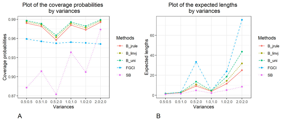
Figure 3: Graphs to compare the performance of the proposed methods in terms of (A) coverage probability (B) expected length with varying variances.

Download full-size image

DOI: 10.7717/peerj.9662/fig-3

Table 1:

The coverage probabilities and expected lengths of 95% confidence intervals for the difference CVs.

n₁:n₂	δ₁:δ₂	σ₁²:σ₂²	Coverage probabilities (Expected lengths)
n₁:n₂	δ₁:δ₂	σ₁²:σ₂²	FGCI	B_linvj	B_jrule	B_uni	SB
25:25	0.5:0.5	0.5:0.5	0.9673	0.9973	0.9966	0.9979	0.8869
			(2.1594)	(2.2567)	(2.0837)	(2.4013)	(1.0054)
		0.5:1.0	0.9559	0.9889	0.9843	0.9913	0.8613
			(4.6245)	(4.1756)	(3.7971)	(4.5568)	(1.9066)
		0.5:2.0	0.9533	0.9627	0.9529	0.9699	0.7995
			(33.3988)	(19.2637)	(16.7548)	(22.7213)	(7.2489)
		1.0:1.0	0.9573	0.9976	0.9957	0.9984	0.9555
			(6.8460)	(6.4599)	(5.7927)	(7.1950)	(2.5935)
		1.0:2.0	0.9530	0.9793	0.9732	0.9845	0.8525
			(35.1495)	(21.5802)	(18.6556)	(25.3295)	(8.2679)
		2.0:2.0	0.9517	0.9983	0.9969	0.9989	0.9913
			(68.0825)	(45.4033)	(37.8180)	(54.8612)	(11.6755)
	0.8:0.8	0.5:0.5	0.9567	0.9861	0.9827	0.9889	0.9183
			(1.2510)	(1.2894)	(1.2393)	(1.3425)	(0.8089)
		0.5:1.0	0.9523	0.9785	0.9751	0.9836	0.9056
			(2.3240)	(2.2129)	(2.1182)	(2.3214)	(1.4044)
		0.5:2.0	0.9522	0.9608	0.9537	0.9651	0.8502
			(9.5540)	(7.3571)	(6.9618)	(7.8340)	(4.5031)
		1.0:1.0	0.9511	0.9889	0.9848	0.9899	0.9567
			(3.2549)	(3.1689)	(3.0159)	(3.3480)	(1.8576)
		1.0:2.0	0.9529	0.9753	0.9720	0.9796	0.8833
			(10.1630)	(8.2686)	(7.7973)	(8.8496)	(4.6834)
		2.0:2.0	0.9477	0.9940	0.9928	0.9959	0.9917
			(3.0485)	(14.5891)	(13.6002)	(15.7798)	(6.8311)
25:50	0.5:0.5	0.5:0.5	0.9624	0.9901	0.9863	0.9921	0.8592
			(1.7255)	(1.7888)	(1.6832)	(1.8646)	(0.8931)
		0.5:1.0	0.9599	0.9909	0.9899	0.9929	0.9269
			(2.5974)	(2.6381)	(2.4939)	(2.7539)	(1.5072)
		0.5:2.0	0.9509	0.9686	0.9642	0.9721	0.8709
			(8.1783)	(7.0822)	(6.7312)	(7.3973)	(4.5482)
		1.0:1.0	0.9549	0.9903	0.9867	0.9921	0.9263
			(4.9820)	(4.5559)	(4.2090)	(4.9041)	(2.2435)
		1.0:2.0	0.9561	0.9877	0.9855	0.9907	0.9216
			(10.1142)	(9.3743)	(8.7358)	(10.0319)	(5.0513)
		2.0:2.0	0.9522	0.9918	0.9900	0.9929	0.9769
			(37.8763)	(26.1295)	(22.8554)	(30.0308)	(9.3159)
	0.8:0.8	0.5:0.5	0.9528	0.9811	0.9776	0.9841	0.9013
			(1.0224)	(1.0467)	(1.0148)	(1.0790)	(0.7012)
		0.5:1.0	0.9531	0.9805	0.9774	0.9817	0.9360
			(1.5016)	(1.5188)	(1.4793)	(1.5628)	(1.0872)
		0.5:2.0	0.9533	0.9633	0.9609	0.9651	0.9000
			(4.1192)	(3.7823)	(3.6962)	(3.8776)	(2.9613)
		1.0:1.0	0.9512	0.9812	0.9773	0.9845	0.9398
			(2.5113)	(2.4208)	(2.3346)	(2.5203)	(1.6020)
		1.0:2.0	0.9528	0.9772	0.9745	0.9801	0.9347
			(4.8629)	(4.6740)	(4.5325)	(4.8398)	(3.2412)
		2.0:2.0	0.9508	0.9871	0.9841	0.9898	0.9751
			(11.2886)	(9.8332)	(9.3589)	(10.4176)	(5.6187)
25:100	0.5:0.5	0.5:0.5	0.9603	0.9811	0.9749	0.9832	0.7991
			(1.5388)	(1.5690)	(1.4780)	(1.6325)	(0.8035)
		0.5:1.0	0.9587	0.9885	0.9850	0.9899	0.9285
			(1.9519)	(2.0049)	(1.9077)	(2.0801)	(1.1956)
		0.5:2.0	0.9522	0.9769	0.9743	0.9787	0.9147
			(4.4100)	(4.2612)	(4.1242)	(4.3739)	(3.1908)
		1.0:1.0	0.9537	0.9771	0.9696	0.9802	0.8726
			(4.5423)	(3.8597)	(3.5765)	(4.1514)	(2.0158)
		1.0:2.0	0.9530	0.9913	0.9887	0.9926	0.9609
			(6.5209)	(6.1550)	(5.8006)	(6.5196)	(3.6771)
		2.0:2.0	0.9508	0.9789	0.9729	0.9825	0.9217
			(36.2420)	(21.8964)	(19.2432)	(25.4336)	(8.1490)
	0.8:0.8	0.5:0.5	0.9539	0.9764	0.9719	0.9824	0.8773
			(0.9261)	(0.9326)	(0.9045)	(0.9614)	(0.6381)
		0.5:1.0	0.9533	0.9767	0.9749	0.9793	0.9374
			(1.1685)	(1.1851)	(1.1561)	(1.2151)	(0.8741)
		0.5:2.0	0.9526	0.9672	0.9655	0.9688	0.9323
			(2.5254)	(2.4766)	(2.4398)	(2.5174)	(2.0893)
		1.0:1.0	0.9503	0.9721	0.9685	0.9769	0.9051
			(2.2790)	(2.1192)	(2.0446)	(2.2031)	(1.4489)
		1.0:2.0	0.9537	0.9805	0.9788	0.9827	0.9623
			(3.3455)	(3.2986)	(3.2136)	(3.3991)	(2.4324)
		2.0:2.0	0.9515	0.9759	0.9736	0.9790	0.9254
			(10.1643)	(8.1980)	(7.8121)	(8.6649)	(4.9982)
50:50	0.2:0.2	0.5:0.5	0.9687	0.9990	0.9987	0.9993	0.8457
			(4.3446)	(4.4760)	(3.9330)	(4.8772)	(1.5117)
		0.5:1.0	0.9596	0.9938	0.9909	0.9955	0.8318
			(11.3576)	(9.2035)	(7.8085)	(10.6120)	(3.0407)
		0.5:2.0	0.9527	0.9628	0.9497	0.9692	0.7672
			(379.5699)	(68.3314)	(50.3354)	(102.5227)	(13.8885)
		1.0:1.0	0.9589	0.9995	0.9991	0.9997	0.9505
			(17.8892)	(14.9444)	(12.3859)	(17.8983)	(4.2541)
		1.0:2.0	0.9535	0.9846	0.9763	0.9889	0.8213
			(221.5949)	(102.3997)	(68.1067)	(157.6987)	(13.9408)
		2.0:2.0	0.9527	0.9995	0.9987	0.9996	0.9905
			(687.4366)	(183.4749)	(127.6218)	(282.3258)	(22.4336)
	0.5:0.5	0.5:0.5	0.9609	0.9921	0.9904	0.9929	0.8980
			(1.2063)	(1.3303)	(1.2870)	(1.3520)	(0.7659)
		0.5:1.0	0.9561	0.9815	0.9789	0.9829	0.8954
			(2.1991)	(2.1818)	(2.1051)	(2.2345)	(1.4150)
		0.5:2.0	0.9528	0.9573	0.9526	0.9599	0.8577
			(7.8990)	(6.6471)	(6.3821)	(6.8773)	(4.6165)
		1.0:1.0	0.9559	0.9888	0.9879	0.9914	0.9531
			(3.0060)	(2.9998)	(2.8860)	(3.0909)	(1.8965)
		1.0:2.0	0.9527	0.9725	0.9679	0.9751	0.8837
			(8.5000)	(7.4233)	(7.1057)	(7.6981)	(4.7694)
		2.0:2.0	0.9514	0.9937	0.9930	0.9954	0.9889
			(13.1899)	(12.1455)	(11.5553)	(12.6939)	(6.8683)
50:50	0.8:0.8	0.5:0.5	0.9537	0.9793	0.9785	0.9815	0.9224
			(0.7572)	(0.7973)	(0.7838)	(0.8097)	(0.5878)
		0.5:1.0	0.9521	0.9677	0.9651	0.9700	0.9216
			(1.2943)	(1.2861)	(1.2634)	(1.3091)	(1.0115)
		0.5:2.0	0.9519	0.9565	0.9547	0.9589	0.8909
			(4.0145)	(3.5922)	(3.5249)	(3.6685)	(2.9205)
		1.0:1.0	0.9513	0.9759	0.9736	0.9787	0.9513
			(1.7224)	(1.7283)	(1.6967)	(1.7633)	(1.3158)
		1.0:2.0	0.9521	0.9641	0.9613	0.9670	0.9110
			(4.2510)	(3.9321)	(3.8539)	(4.0204)	(3.0627)
		2.0:2.0	0.9523	0.9865	0.9844	0.9870	0.9845
			(6.2427)	(6.0484)	(5.9146)	(6.2018)	(4.2865)
50:100	0.2:0.2	0.5:0.5	0.9640	0.9964	0.9941	0.9964	0.8360
			(3.2908)	(3.3693)	(3.0608)	(3.5439)	(1.3380)
		0.5:1.0	0.9623	0.9969	0.9956	0.9977	0.9038
			(4.9483)	(5.0554)	(4.6240)	(5.3501)	(2.3793)
		0.5:2.0	0.9552	0.9701	0.9655	0.9738	0.8367
			(17.1227)	(14.0971)	(12.9842)	(14.9740)	(7.8643)
		1.0:1.0	0.9587	0.9956	0.9930	0.9968	0.9299
			(11.9262)	(9.6133)	(8.4150)	(10.8005)	(3.6621)
		1.0:2.0	0.9534	0.9909	0.9869	0.9931	0.8973
			(22.9239)	(20.1401)	(17.9128)	(22.3911)	(8.7065)
		2.0:2.0	0.9509	0.9954	0.9919	0.9966	0.9803
			(206.9601)	(100.4277)	(72.9777)	(157.2391)	(18.0215)
	0.5:0.5	0.5:0.5	0.9596	0.9859	0.9845	0.9875	0.8779
			(1.0067)	(1.1041)	(1.0756)	(1.1170)	(0.6672)
		0.5:1.0	0.9532	0.9823	0.9816	0.9836	0.9266
			(1.4826)	(1.5699)	(1.5343)	(1.5906)	(1.0971)
		0.5:2.0	0.9503	0.9615	0.9590	0.9637	0.9013
			(4.0903)	(3.8417)	(3.7690)	(3.8933)	(3.1255)
		1.0:1.0	0.9525	0.9801	0.9776	0.9827	0.9359
			(2.3930)	(2.3893)	(2.3204)	(2.4426)	(1.6419)
		1.0:2.0	0.9524	0.9768	0.9756	0.9799	0.9319
			(4.6910)	(4.5889)	(4.4772)	(4.6767)	(3.4066)
		2.0:2.0	0.9501	0.9829	0.9803	0.9847	0.9723
			(9.6921)	(8.9658)	(8.6364)	(9.2571)	(5.7747)
	0.8:0.8	0.5:0.5	0.9509	0.9723	0.9706	0.9763	0.9179
			(0.6389)	(0.6704)	(0.6613)	(0.6788)	(0.5113)
		0.5:1.0	0.9507	0.9697	0.9678	0.9702	0.9416
			(0.9307)	(0.9511)	(0.9404)	(0.9619)	(0.7815)
		0.5:2.0	0.9533	0.9577	0.9570	0.9595	0.9261
			(2.3889)	(2.2905)	(2.2691)	(2.3127)	(2.0442)
		1.0:1.0	0.9535	0.9701	0.9678	0.9722	0.9411
			(1.4198)	(1.4116)	(1.3911)	(1.4335)	(1.1429)
		1.0:2.0	0.9513	0.9679	0.9667	0.9693	0.9441
			(2.6872)	(2.6428)	(2.6126)	(2.6764)	(2.2221)
		2.0:2.0	0.9505	0.9757	0.9742	0.9783	0.9665
			(4.9394)	(4.7304)	(4.6503)	(4.8203)	(3.6171)
100:100	0.2:0.2	0.5:0.5	0.9669	0.9954	0.9950	0.9959	0.8686
			(2.1090)	(2.3784)	(2.2658)	(2.4068)	(1.1520)
		0.5:1.0	0.9562	0.9871	0.9826	0.9881	0.8686
			(3.9894)	(3.9890)	(3.7803)	(4.0876)	(2.2483)
		0.5:2.0	0.9513	0.9582	0.9510	0.9615	0.8265
			(16.4620)	(12.9759)	(12.1641)	(13.5255)	(7.9611)
		1.0:1.0	0.9571	0.9943	0.9941	0.9961	0.9517
			(5.5425)	(5.6080)	(5.2895)	(5.7983)	(3.0592)
		1.0:2.0	0.9538	0.9755	0.9709	0.9775	0.8632
			(17.6427)	(14.6645)	(13.7125)	(15.3659)	(8.2895)
		2.0:2.0	0.9523	0.9963	0.9953	0.9971	0.9896
			(27.9500)	(25.3838)	(23.5151)	(26.9001)	(12.1880)
	0.5:0.5	0.5:0.5	0.9564	0.9865	0.9853	0.9874	0.9045
			(0.7720)	(0.8662)	(0.8530)	(0.8708)	(0.5607)
		0.5:1.0	0.9570	0.9731	0.9703	0.9740	0.9140
			(1.3204)	(1.3613)	(1.3402)	(1.3733)	(1.0281)
		0.5:2.0	0.9503	0.9549	0.9525	0.9559	0.8907
			(4.0361)	(3.6979)	(3.6367)	(3.7426)	(3.1053)
		1.0:1.0	0.9518	0.9779	0.9761	0.9792	0.9519
			(1.7362)	(1.7898)	(1.7605)	(1.8090)	(1.3591)
		1.0:2.0	0.9511	0.9643	0.9619	0.9654	0.9125
			(4.2295)	(4.0091)	(3.9418)	(4.0614)	(3.2737)
		2.0:2.0	0.9505	0.9833	0.9811	0.9843	0.9809
			(6.1135)	(6.0198)	(5.9072)	(6.1094)	(4.5458)
	0.8:0.8	0.5:0.5	0.9531	0.9719	0.9719	0.9734	0.9296
			(0.5013)	(0.5311)	(0.5269)	(0.5348)	(0.4237)
		0.5:1.0	0.9511	0.9643	0.9625	0.9653	0.9302
			(0.8306)	(0.8394)	(0.8328)	(0.8460)	(0.7232)
		0.5:2.0	0.9525	0.9505	0.9495	0.9521	0.9194
			(2.3561)	(2.2276)	(2.2088)	(2.2473)	(2.0198)
		1.0:1.0	0.9529	0.9641	0.9618	0.9653	0.9511
			(1.0792)	(1.0925)	(1.0835)	(1.1015)	(0.9386)
		1.0:2.0	0.9534	0.9614	0.9606	0.9637	0.9299
			(2.4814)	(2.3968)	(2.3755)	(2.4182)	(2.1126)
		2.0:2.0	0.9521	0.9729	0.9710	0.9742	0.9747
			(3.4679)	(3.4336)	(3.4027)	(3.4682)	(2.8902)

DOI: 10.7717/peerj.9662/table-1

The empirical study

Datasets of rainfall from Thailand were chosen because they usually contain zero values, albeit data containing non-zero values normally follow a lognormal distribution. For rainfall data, Ananthakrishnan & Soman (1989) used the normalized rainfall curve (NRC) to describe the relationship between the accumulated percentage of the rain amount and the number of rain days in a rainfall series. Their results indicate that the coefficient of variation of the rainfall datasets can be used in the unique determination of the NRC. Moreover, Shimizu (1993) introduced a probability model for a combination of bivariate and lognormal distributions to represent rainfall data. The author used monthly rainfall data from Jana and Ranod, Songkhla, Thailand from 2008 to 2017 to illustrate confidence intervals for the difference between coefficients of variation from two areas.

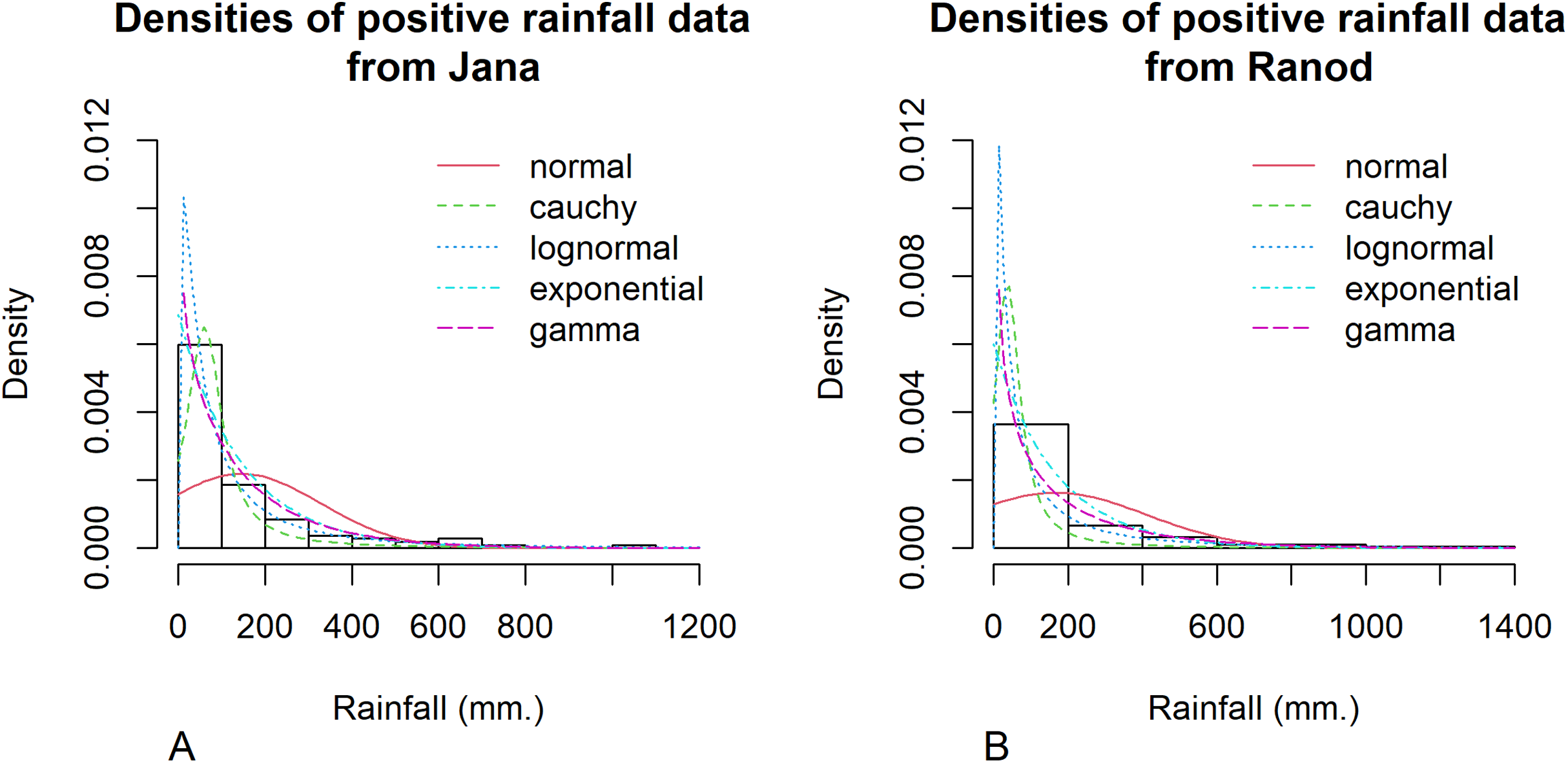
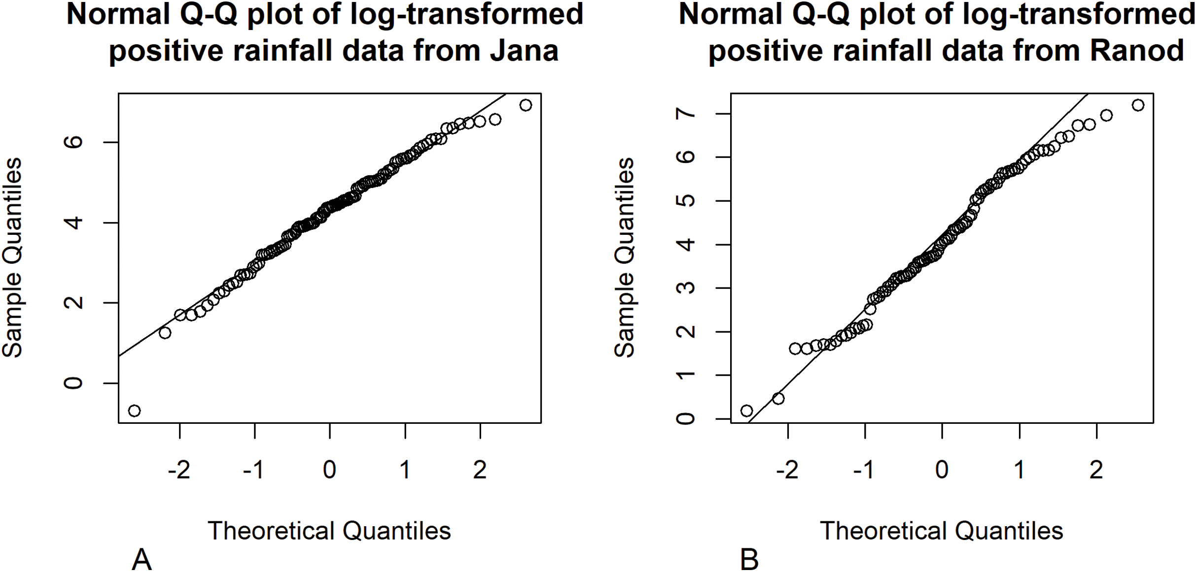
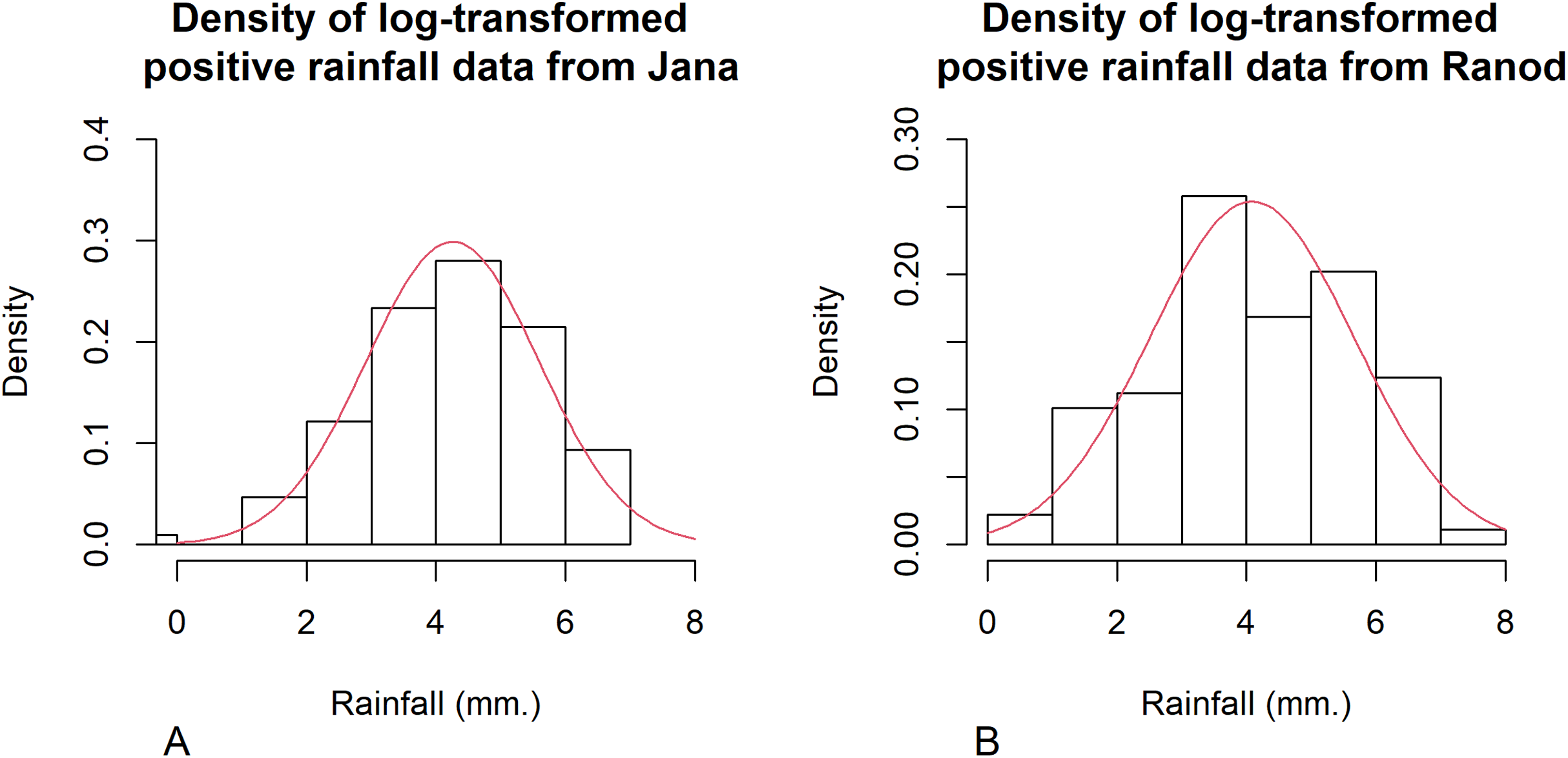
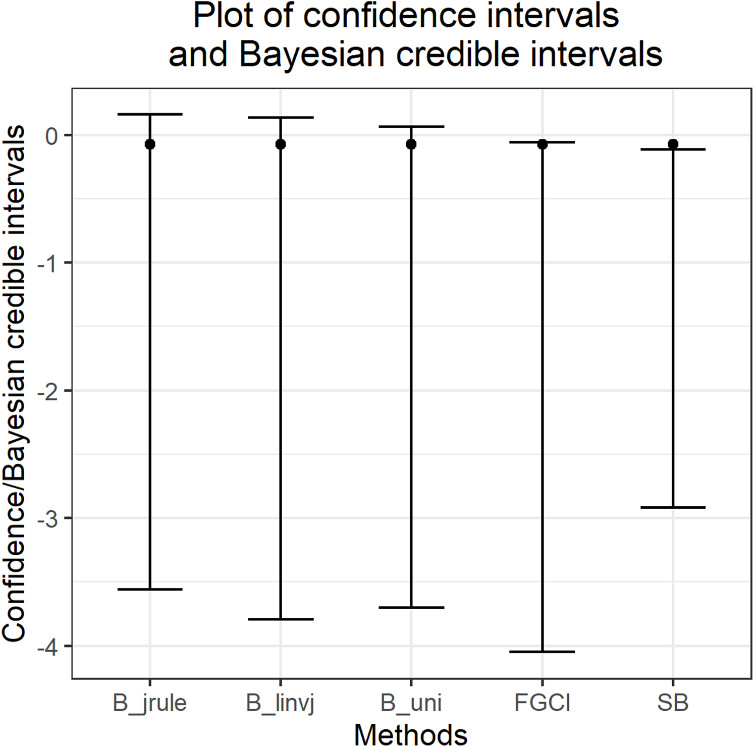
Songkhla is located on the east coast of southern Thailand and is somewhat rainy due to the influences of the southwest monsoon coming from the Indian Ocean and the northeast monsoon coming from the Gulf of Thailand. This area has a lot of rain from May to December, which decreases from January to April (the datasets were collected by the Southern Meteorological Center (East Coast)). These datasets included both positive and true-zero observations. The positive values for each area create skewness, as shown in Fig. 4, and thus their distributions were subjected to Akaike information criterion (AIC) analyses. The AIC values according to normal, Cauchy, lognormal, exponential, and gamma distributions in Jana were 1421.5050, 1355.5600, 1279.9710, 1281.8810, and 1280.7610 and in Ranod were 1234.7680, 1155.3230, 1063.9270, 1090.1390, and 1073.1520, respectively. The AIC values indicating a lognormal distribution were less than the others, and so the positive datasets from Jana and Ranod are lognormal distributions. To confirm AIC results, the normality plots of the log-transformation of the monthly rainfall data from both areas in Figs. 5 and 6 indicate that both rainfall series are lognormal distributions. Moreover, the true-zero values from Jana and Ranod are binomial distributions. Therefore, the distributions of the monthly rainfall series from Jana and Ranod are delta-lognormal. The summary statistics for Jana are n₁ = 120, ${\hat{δ}}_{1} = 0.8917$ , ${\hat{μ}}_{1} = 4.2556$ , ${\hat{σ}}_{1}^{2} = 1.7953$ , and ${\hat{η}}_{1} = 0.3149$ and for Ranod are n₂ = 120, ${\hat{δ}}_{2} = 0.7417$ , ${\hat{μ}}_{2} = 4.0846$ , ${\hat{σ}}_{2}^{2} = 2.4928$ , and ${\hat{η}}_{2} = 0.3865$ . The difference between ${\hat{η}}_{1}$ and ${\hat{η}}_{2}$ is γ = − 0.0716. The 95% confidence intervals for FGCI and SB are (−4.0492, −0.0558), and (−2.9163, −0.1118) with interval lengths of 3.9934 and 2.8045, respectively. Similarly, the 95% Bayesian HPD intervals using the left-invariant Jeffreys, Jeffreys’ Rule, and uniform priors are (−3.7924, 0.1359), (−3.5602, 0.1619), and (−3.7008, 0.0646) with interval lengths 3.9283, 3.7221, and 3.7654, respectively. These intervals are shown in Fig. 7. The Bayesian method using the Jeffreys’ Rule prior outperformed the others in terms of the coverage probability and interval length. Therefore, these results are in accordance with those from the simulation studies when the variance is large. Furthermore, the results for the Bayesian method using the Jeffreys’ Rule prior demonstrate that there is not a difference in the rainfall intensity between the areas.

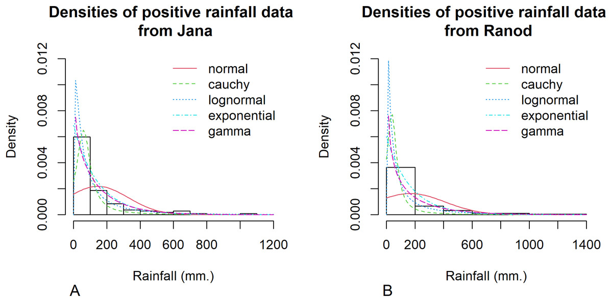
Figure 4: Histogram and theoretical densities of the positive monthly rainfall data from (A) Jana (B) Ranod, Songkhla, Thailand from 2008 to 2017.

Download full-size image

DOI: 10.7717/peerj.9662/fig-4

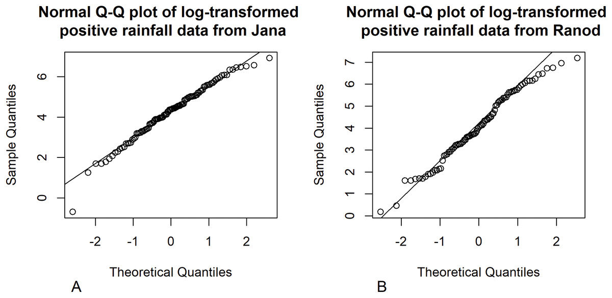
Figure 5: Normal Q–Q plots of the log-transformed positive monthly rainfall data from (A) Jana (B) Ranod, Songkhla, Thailand from 2008 to 2017.

Download full-size image

DOI: 10.7717/peerj.9662/fig-5

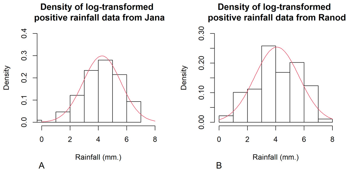
Figure 6: Histogram and theoretical density of the log-transformed positive monthly rainfall data from (A) Jana (B) Ranod, Songkhla, Thailand from 2008 to 2017.

Download full-size image

DOI: 10.7717/peerj.9662/fig-6

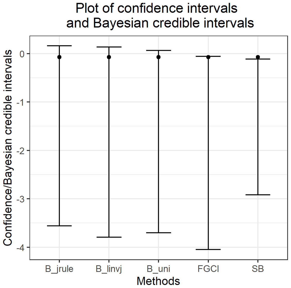
Figure 7: The 95% confidence intervals and Bayesian credible intervals for the difference between coefficients of variation of the monthly rainfall data from Jana and Ranod, Songkhla, Thailand from 2008 to 2017.

Download full-size image

DOI: 10.7717/peerj.9662/fig-7

Discussion

Herein, Bayesian and SB methods are proposed to construct confidence intervals for the difference between delta-lognormal coefficients of variation and then compared with FGCI recommended by Yosboonruang, Niwitpong & Niwitpong (2019a). It was found that the coverage probabilities of FGCI were more consistent with the target than the Bayesian and SB methods. The coverage probabilities of the Bayesian method were greater than the nominal confidence level and mostly close to 1.00, which suggests overestimation. Nevertheless, the expected lengths of the Bayesian method using the Jeffreys’ Rule prior were shorter than FGCI in almost every case. This is due to the criterion that the posterior density values at the lower and upper limits are equal, which was applied for constructing the confidence intervals of the Bayesian methods. Moreover, in case of small variances, it is notable that the expected lengths of the confidence intervals were sufficiently narrow. This indicated that FGCI and the Bayesian methods can be efficiently used to construct the confidence intervals. Furthermore, the coverage probabilities of the SB method were greater than the nominal confidence level only for the large variance cases, although remarkably, it supplied the shortest expected lengths. However, these three methods required a large amount of computing to obtain the interval estimates due to FGCI must be calculated GFQ for parameters of interest (δ_i and $σ_{i}^{2}$ ) and the Bayesian method must be obtained the posterior densities of ${\tilde{δ}}_{i}$ and $σ_{i}^{2}$ . In addition, SB method have to resample bootstrap samples for computing the estimators of δ_i and $σ_{i}^{2}$ which takes more time than FGCI and the Bayesian methods. The results using the two rainfall data series were matched with the simulation, with the Bayesian method using the Jeffreys’ Rule prior demonstrating the difference between their coefficients of variation much better than the others.

Conclusions

In this study, the three concepts: FGCI, Bayesian, and SB methods were used to construct five confidence intervals for the difference between two independent coefficients of variation of a delta-lognormal distribution. Of these, the Bayesian method was used to construct three confidence intervals using the left-invariant Jeffreys, Jeffreys’ Rule, and uniform priors under HPD intervals. Other confidence intervals based on the SB method and FGCI were also used.

The results of the simulation studies indicate that the performance of the Bayesian HPD based on the Jeffreys’ Rule prior performed the best in almost all cases. Although the coverage probabilities were close to 1.00 for all of the priors, the expected lengths of the Jeffreys’ Rule prior were shorter for the confidence intervals of the difference between the coefficients of variation of two delta-lognormal distributions in almost all cases. Moreover, FGCI is appropriate for a large sample size together with small variance while the SB method is suggested for a large variance. Furthermore, a comparison of the simulation results and using sets of real data indicates that the Bayesian method using the Jeffreys’ Rule prior can be recommended for constructing the confidence intervals for the difference between two independent coefficients of variation of a delta-lognormal distribution.

Supplemental Information

R code.

DOI: 10.7717/peerj.9662/supp-1

Download

Monthly rainfall data (mm.) measuring from Jana, Songkhla, Thailand from 2008 to 2017.

DOI: 10.7717/peerj.9662/supp-2

Download

Monthly rainfall data (mm.) measuring from Ranod, Songkhla, Thailand from 2008 to 2017.

DOI: 10.7717/peerj.9662/supp-3

Download

[1] Aitchison J. 1955. On the distribution of a positive random variable having a discrete probability mass at the origin. Journal of the American Statistical Association 50:901-908

[2] Aldrich J. 2000. Fisher’s “inverse probability” of 1930. International Statistical Review 68(2):155-172

[3] Ananthakrishnan R, Soman M. 1989. Statistical distribution of daily rainfall and its association with the coefficient of variation of rainfall series. International Journal of Climatology 9(5):485-500

[4] Attavanich W. 2013. The effect of climate change on Thailand’s agriculture.

[5] Bolstad WM, Curran JM. 2017. Introduction to Bayesian statistics (Third Edition). Hoboken: John Wiley & Sons.

[6] Buntao N, Niwitpong S-A. 2012. Confidence intervals for the difference of coefficients of variation for lognormal distributions and delta-lognormal distributions. Applied Mathematical Sciences 6(134):6691-6704

[7] Buntao N, Niwitpong S-A. 2013. Confidence intervals for the ratio of coefficients of variation of delta-lognormal distribution. Applied Mathematical Sciences 7(77):3811-3818

[8] Chen Y-H, Zhou X-H. 2006. Generalized confidence intervals for the ratio or difference of two means for lognormal populations with zeros. UW Biostatistics Working Paper Series. Working Paper 296

[9] Dawid AP, Stone M. 1982. The functional-model basis of fiducial inference. Annals of Statistics 10(4):1054-1067

[10] Donner A, Zou GY. 2012. Closed-form confidence intervals for functions of the normal mean and standard deviation. Statistical Methods in Medical Research 21(4):347-359

[11] Efron B. 1979. Bootstrap methods: another look at the Jackknife. Annals of Statistics 7(1):1-26

[12] Eso M, Kuning M, Chuai-Aree S. 2015. Analysis of daily rainfall during 2001–2012 in Thailand. Songklanakarin Journal of Science and Technology 37(1):81-88

[13] Fisher RA. 1930. Inverse probability. Mathematical Proceedings of the Cambridge Philosophical Society 26(4):528-535

[14] Fletcher D. 2008. Confidence intervals for the mean of the delta-lognormal distribution. Environmental and Ecological Statistics 15(2):175-189

[15] Fukuchi H. 1988. Correlation properties of rainfall rates in the United Kingdom. Antennas and Propagation IEE Proceedings H: Microwaves 135(2):83-88

[16] Hannig J. 2009. On generalized fiducial inference. Statistica Sinica 19(2):491-544

[17] Hannig J, Lidong E, Abdel-Karim A, Iyer H. 2006. Simultaneous fiducial generalized confidence intervals for ratios of means of lognormal distributions. Austrian Journal of Statistics 35(2&3):261-269

[18] Hannig J, Iyer H, Patterson P. 2006. Fiducial generalized confidence intervals. Journal of the American Statistical Association 101(473):254-269

[19] Hannig J, Lee TCM. 2009. Generalized fiducial inference for wavelet regression. Biometrika 96(4):847-860

[20] Harvey J, Van der Merwe AJ. 2012. Bayesian confidence intervals for means and variances of lognormal and bivariate lognormal distributions. Journal of Statistical Planning and Inference 142(6):1294-1309

[21] Kalkur TA, Rao A. 2017. Bayes estimator for coefficient of variation and inverse coefficient of variation for the normal distribution. International Journal of Statistics and Systems 12(4):721-732

[22] Kong CY, Jamaludin S, Yusof F, Foo HM. 2012. Parameter estimation for bivariate mixed lognormal distribution. Journal of Science and Technology 4(1):41-48

[23] Li X, Zhou X, Tian L. 2013. Interval estimation for the mean of lognormal data with excess zeros. Statistics & Probability Letters 83(11):2447-2453

[24] Maneerat P, Niwitpong S-A, Niwitpong S. 2018. Confidence intervals for the ratio of means of delta-lognormal distribution. In: Anh LH, Dong LS, Kreinovich V, Thach NN, eds. Econometrics for Financial Applications, Studies in Computational Intelligence. Cham: Springer International Publishing. 161-174

[25] Maneerat P, Niwitpong S-A, Niwitpong S. 2019a. Bayesian confidence intervals for a single mean and the difference between two means of delta-lognormal distributions. Communications in Statistics—Simulation and Computation 0(0):1-29

[26] Maneerat P, Niwitpong S-A, Niwitpong S. 2019b. Confidence intervals for the mean of delta-lognormal distribution. In: Kreinovich V, Sriboonchitta S, eds. Structural Changes and their Econometric Modeling, Studies in Computational Intelligence. Cham: Springer International Publishing. 264-274

[27] Niwitpong S-A. 2015. Confidence intervals for the difference between coefficients of variation of normal distribution with bounded parameters. Far East Journal of Mathematical Sciences 98(5):649-663

[28] Rao KA, D’Cunha JG. 2016. Bayesian inference for median of the lognormal distribution. Journal of Modern Applied Statistical Methods 15(2):526-535

[29] Sangnawakij P, Niwitpong S-A. 2017a. Confidence intervals for coefficients of variation in two-parameter exponential distributions. Communications in Statistics—Simulation and Computation 46(8):6618-6630

[30] Sangnawakij P, Niwitpong S-A. 2017b. Confidence intervals for functions of coefficients of variation with bounded parameter spaces in two gamma distributions. Songklanakarin Journal of Science and Technology 39(1):27-39

[31] Shimizu K. 1993. A bivariate mixed lognormal distribution with an analysis of rainfall data. Journal of Applied Meteorology 32(2):161-171

[32] Thangjai W, Niwitpong S-A. 2017. Confidence intervals for the weighted coefficients of variation of two-parameter exponential distributions. Cogent Mathematics 4(1):1315880

[33] Tian L. 2005. Inferences on the mean of zero-inflated lognormal data: the generalized variable approach. Statistics in Medicine 24(20):3223-3232

[34] Tian L, Wu J. 2006. Confidence intervals for the mean of lognormal data with excess zeros. Biometrical Journal. Biometrische Zeitschrift 48(1):149-156

[35] Wong ACM, Wu J. 2002. Small sample asymptotic inference for the coefficient of variation: normal and nonnormal models. Journal of Statistical Planning and Inference 104(1):73-82

[36] Wongkhao A, Niwitpong S-A, Niwitpong S. 2015. Confidence intervals for the ratio of two independent coefficients of variation of normal distribution. Far East Journal of Mathematical Sciences 98(6):741-757

[37] Wu W-H, Hsieh H-N. 2014. Generalized confidence interval estimation for the mean of delta-lognormal distribution: an application to New Zealand trawl survey data. Journal of Applied Statistics 41(7):1471-1485

[38] Yosboonruang N, Niwitpong S, Niwitpong S-A. 2019a. Confidence intervals for coefficient of variation of three parameters delta-lognormal distribution. In: Kreinovich V, Sriboonchitta S, eds. Structural Changes and their Econometric Modeling, Studies in Computational Intelligence. Cham: Springer International Publishing. 352-363