
Visualising higher-dimensional space-time and space-scale objects as projections to ℝ3
- Published
- Accepted
- Received
- Academic Editor
- Sándor Szénási
- Subject Areas
- Graphics, Scientific Computing and Simulation, Spatial and Geographic Information Systems
- Keywords
- Projections, Space-time, Space-scale, 4D visualisation, Nd gis
- Copyright
- © 2017 Arroyo Ohori et al.
- Licence
- This is an open access article distributed under the terms of the Creative Commons Attribution License, which permits unrestricted use, distribution, reproduction and adaptation in any medium and for any purpose provided that it is properly attributed. For attribution, the original author(s), title, publication source (PeerJ Computer Science) and either DOI or URL of the article must be cited.
- Cite this article
- 2017. Visualising higher-dimensional space-time and space-scale objects as projections to ℝ3. PeerJ Computer Science 3:e123 https://doi.org/10.7717/peerj-cs.123
Abstract
Objects of more than three dimensions can be used to model geographic phenomena that occur in space, time and scale. For instance, a single 4D object can be used to represent the changes in a 3D object’s shape across time or all its optimal representations at various levels of detail. In this paper, we look at how such higher-dimensional space-time and space-scale objects can be visualised as projections from ℝ4 to ℝ3. We present three projections that we believe are particularly intuitive for this purpose: (i) a simple ‘long axis’ projection that puts 3D objects side by side; (ii) the well-known orthographic and perspective projections; and (iii) a projection to a 3-sphere (S3) followed by a stereographic projection to ℝ3, which results in an inwards-outwards fourth axis. Our focus is in using these projections from ℝ4 to ℝ3, but they are formulated from ℝn to ℝn−1 so as to be easily extensible and to incorporate other non-spatial characteristics. We present a prototype interactive visualiser that applies these projections from 4D to 3D in real-time using the programmable pipeline and compute shaders of the Metal graphics API.
Background
Projecting the 3D nature of the world down to two dimensions is one of the most common problems at the juncture of geographic information and computer graphics, whether as the map projections in both paper and digital maps (Snyder, 1987; Grafarend & You, 2014) or as part of an interactive visualisation of a 3D city model on a computer screen (Foley & Nielson, 1992; Shreiner et al., 2013). However, geographic information is not inherently limited to objects of three dimensions. Non-spatial characteristics such as time (Hägerstrand, 1970; Güting et al., 2000; Hornsby & Egenhofer, 2002; Kraak, 2003) and scale (Meijers, 2011a) are often conceived and modelled as additional dimensions, and objects of three or more dimensions can be used to model objects in 2D or 3D space that also have changing geometries along these non-spatial characteristics (Van Oosterom & Stoter, 2010; Arroyo Ohori, 2016). For example, a single 4D object can be used to represent the changes in a 3D object’s shape across time (Arroyo Ohori, Ledoux & Stoter, 2017) orall the best representations of a 3D object at various levels of detail (Luebke et al., 2003; Van Oosterom & Meijers, 2014; Arroyo Ohori et al., 2015a; Arroyo Ohori, Ledoux & Stoter, 2015c).
Objects of more than three dimensions can be however unintuitive (Noll, 1967; Frank, 2014), and visualising them is a challenge. While some operations on a higher-dimensional object can be achieved by running automated methods (e.g. certain validation tests or area/volume computations) or by visualising only a chosen 2D or 3D subset (e.g. some of its bounding faces or a cross-section), sometimes there is no substitute for being able to view a complete nD object—much like viewing floor or façade plans is often no substitute for interactively viewing the complete 3D model of a building. By viewing a complete model, one can see at once the 3D objects embedded in the model at every point in time or scale as well as the equivalences and topological relationships between their constituting elements. More directly, it also makes it possible to get an intuitive understanding of the complexity of a given 4D model.
For instance, in Fig. 1 we show an example of a 4D model representing a house at two different levels of detail and all the equivalences its composing elements. It forms a valid manifold 4-cell (Arroyo Ohori, Damiand & Ledoux, 2014), allowing it to be represented using data structures such as a 4D generalised or combinatorial map.
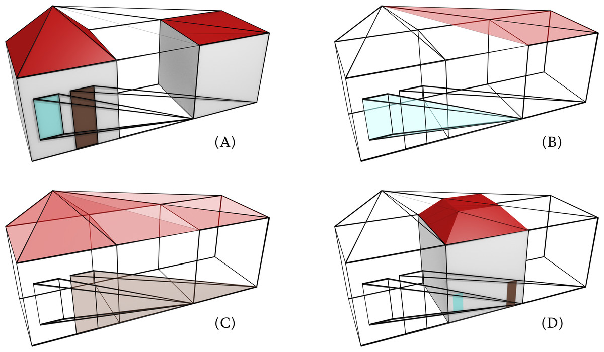
Figure 1: A 4D model of a house at two levels of detail and all the equivalences its composing elements is a polychoron bounded by: (A) volumes representing the house at the two levels of detail, (B) a pyramidal volume representing the window at the higher LOD collapsing to a vertex at the lower LOD, (C) a pyramidal volume representing the door at the higher LOD collapsing to a vertex at the lower LOD, and a roof volume bounded by (A) the roof faces of the two LODs, (B) the ridges at the lower LOD collapsing to the tip at the higher LOD and (C) the hips at the higher LOD collapsing to the vertex below them at the lower LOD. (D) A 3D cross-section of the model obtained at the middle point along the LOD axis.
This paper thus looks at a key aspect that allows higher-dimensional objects to be visualised interactively, namely how to project higher-dimensional objects down to fewer dimensions. While there is previous research on the visualisation of higher-dimensional objects, we aim to do so in a manner that is reasonably intuitive, implementable and fast. We therefore discuss some relevant practical concerns, such as how to also display edges and vertices and how to use compute shaders to achieve good framerates in practice.
In order to do this, we first briefly review the most well-known transformations (translation, rotation and scale) and the cross-product in nD, which we use as fundamental operations in order to project objects and to move around the viewer in an nD scene. Afterwards, we show how to apply three different projections from ℝn to ℝn−1 and argue why we believe they are intuitive enough for real-world use. These can be used to project objects from ℝ4 to ℝ3, and if necessary, they can be used iteratively in order to bring objects of any dimension down to 3D or 2D. We thus present: (i) a simple ‘long axis’ projection that stretches objects along one custom axis while preserving all other coordinates, resulting in 3D objects that are presented side by side; (ii) the orthographic and perspective projections, which are analogous to those used from 3D to 2D; and (iii) an inwards/outwards projection to an (n − 1)-sphere followed by an stereographic projection to ℝn−1, which results in a new inwards-outwards axis.
We present a prototype that applies these projections from 4D to 3D and then applies a standard perspective projection down to 2D. We also show that with the help of low-level graphics APIs, all the required operations can be applied at interactive framerates for the 4D to 3D case. We finish with a discussion of the advantages and disadvantages of this approach.
Higher-dimensional modelling of space, time and scale
There are a great number of models of geographic information, but most consider space, time and scale separately. For instance, space can be modelled using primitive instancing (Foley et al., 1995; Kada, 2007), constructive solid geometry (Requicha & Voelcker, 1977) or various boundary representation approaches (Muller & Preparata, 1978; Guibas & Stolfi, 1985; Lienhardt, 1994), among others. Time can be modelled on the basis of snapshots (Armstrong, 1988; Hamre, Mughal & Jacob, 1997), space–time composites (Peucker & Chrisman, 1975; Chrisman, 1983), events (Worboys, 1992; Peuquet, 1994; Peuquet & Duan, 1995), or a combination of all of these (Abiteboul & Hull, 1987; Worboys, Hearnshaw & Maguire, 1990; Worboys, 1994; Wachowicz & Healy, 1994). Scale is usually modelled based on independent datasets at each scale (Buttenfield & DeLotto, 1989; Friis-Christensen & Jensen, 2003; Meijers, 2011b), although approaches to combine them into single datasets (Gröger et al., 2012) or to create progressive and continuous representations also exist (Ballard, 1981; Jones & Abraham, 1986; Günther, 1988; Van Oosterom, 1990; Filho et al., 1995; Rigaux & Scholl, 1995; Plümer & Gröger, 1997; Van Oosterom, 2005).
As an alternative to the all these methods, it is possible to represent any number of parametrisable characteristics (e.g. two or three spatial dimensions, time and scale) as additional dimensions in a geometric sense, modelling them as orthogonal axes such that real-world 0D–3D entities are modelled as higher-dimensional objects embedded in higher-dimensional space. These objects can be consequently stored using higher-dimensionaldata structures and representation schemes Čomić & de Floriani (2012); Arroyo Ohori, Ledoux & Stoter (2015b). Possible approaches include incidence graphs (Rossignac & O’Connor, 1989; Masuda, 1993; Sohanpanah, 1989; Hansen & Christensen, 1993), Nef polyhedra Bieri & Nef (1988), and ordered topological models Brisson (1993); Lienhardt (1994). This is consistent with the basic tenets of n-dimensional geometry (Descartes, 1637; Riemann, 1868) and topology (Poincaré, 1895), which means that it is possible to apply a wide variety of computational geometry and topology methods to these objects.
In a practical sense, 4D topological relationships between 4D objects provide insights that 3D topological relationships cannot (Arroyo Ohori, Boguslawski & Ledoux, 2013). Also, McKenzie, Williamson & Hazelton (2001) contends that weather and groundwater phenomena cannot be adequately studied in less than four dimensions, and Van Oosterom & Stoter (2010) argue that the integration of space, time and scale into a 5D model for GIS can be used to ease data maintenance and improve consistency, as algorithms could detect if the 5D representation of an object is self-consistent and does not conflict with other objects.
Basic transformations and the cross-product in nD
The basic transformations (translation, scale and rotation) have a straightforward definition in n dimensions, which can be used to move and zoom around a scene composed of nD objects. In addition, the n-dimensional cross-product can be used to obtain a new vector that is orthogonal to a set of other n − 1 vectors in ℝn. We use these operations as a base for nD visualisation and are thus described briefly below.
The translation of a set of points in ℝn can be easily expressed as a sum with a vector , or alternatively as a multiplication with a matrix using homogeneous coordinates1 in an (n + 1) × (n + 1) matrix, which is defined as:
Scaling is similarly simple. Given a vector that defines a scale factor per axis (which in the simplest case can be the same for all axes), it is possible to define a matrix to scale an object as:
Rotation is somewhat more complex. Rotations in 3D are often conceptualised intuitively as rotations around the x, y and z axes. However, this view of the matter is only valid in 3D. In higher dimensions, it is necessary to consider instead rotations parallel to a given plane (Hollasch, 1991), such that a point that is continuously rotated (without changing the rotation direction) will form a circle that is parallel to that plane. This view is valid in 2D (where there is only one such plane), in 3D (where a plane is orthogonal to the usually defined axis of rotation) and in any higher dimension. Incidentally, this shows that the degree of rotational freedom in nD is given by the number of possible combinations of two axes (which define a plane) on that dimension (Hanson, 1994), i.e. .
Thus, in a 4D coordinate system defined by the axes x, y, z and w, it is possible to define six 4D rotation matrices, which correspond to the six rotational degrees of freedom in 4D (Hanson, 1994). These respectively rotate points in ℝ4 parallel to the xy, xz, xw, yz, yw and zw planes:
The n-dimensional cross-product is easy to understand by first considering the lower-dimensional cases. In 2D, it is possible to obtain a normal vector to a 1D line as defined by two (different) points p0 and p1, or equivalently a normal vector to a vector from p0 to p1. In 3D, it is possible to obtain a normal vector to a 2D plane as defined by three (non-collinear) points p0, p1 and p2, or equivalently a normal vector to a pair of vectors from p0 to p1 and from p0 to p2. Similarly, in nD it is possible to obtain a normal vector to a (n − 1)D subspace—probably easier to picture as an (n − 1)-simplex—as defined by n linearly independent points p0, p1, …, pn−1, or equivalently a normal vector to a set of n − 1 vectors from p0 to every other point (i.e., p1, p2, …, pn−1) (Massey, 1983; Elduque, 2004).
Hanson (1994) follows the latter explanation using a set of n − 1 vectors all starting from the first point to give an intuitive definition of the n-dimensional cross-product. Assuming that a point pi in ℝn is defined by a tuple of coordinates denoted as and a unit vector along the ith dimension is denoted as , the n-dimensional cross-product of a set of points p0, p1, …, pn−1 can be expressed compactly as the cofactors of the last column in the following determinant:
The components of the normal vector are thus given by the minors of the unit vectors . This vector –like all other vectors—can be normalised into a unit vector by dividing it by its norm .
Previous work on the visualisation of higher-dimensional objects
There is a reasonably extensive body of work on the visualisation of 4D and nD objects, although it is still more often used for its creative possibilities (e.g., making nice-looking graphics) than for practical applications. In literature, visual metaphors of 4D space were already described in the 1880 sin Flatland: A Romance of Many Dimensions (Abbott, 1884) and A New Era of Thought (Hinton, 1888). Other books that treat the topic intuitively include Beyond the Third Dimension: Geometry, Computer Graphics, and Higher Dimensions (Banchoff, 1996) and The Visual Guide To Extra Dimensions: Visualizing The Fourth Dimension, Higher-Dimensional Polytopes, And Curved Hypersurfaces (McMullen, 2008).
In a more concrete computer graphics context, already in the 1960s, Noll (1967) described a computer implementations of the 4D to 3D perspective projection and its application in art (Noll, 1968).
Beshers & Feiner (1988) describe a system that displays animating (i.e. continuously transformed) 4D objects that are rendered in real-time and use colour intensity to provide a visual cue for the 4D depth. It is extended to n dimensions by Feiner & Beshers (1990).
Banks (1992) describes a system that manipulates surfaces in 4D space. It describes interaction techniques and methods to deal with intersections, transparency and the silhouettes of every surface.
Hanson & Cross (1993) describes a high-speed method to render surfaces in 4D space with shading using a 4D light and occlusion, while Hanson (1994) describes much of the mathematics that are necessary for nD visualisation. A more practical implementation is described in Hanson, Ishkov & Ma (1999).
Chu et al. (2009) describe a system to visualise 2-manifolds and 3-manifolds embedded in 4D space and illuminated by 4D light sources. Notably, it uses a custom rendering pipeline that projects tetrahedra in 4D to volumetric images in 3D—analogous to how triangles in 3D that are usually projected to 2D images.
A different possible approach lies in using meaningful 3D cross-sections of a 4D dataset. For instance, Kageyama (2016) describes how to visualise 4D objects as a set of hyperplane slices. Bhaniramka, Wenger & Crawfis (2000) describe how to compute isosurfaces in dimensions higher than three using an algorithm similar to marching cubes. D’Zmura, Colantoni & Seyranian (2000) describe a system that displays 3D cross-sections of a 4D virtual world one at a time.
Similar to the methods described above, Hollasch (1991) gives a simple formulation to describe the 4D to 3D projections, which is itself based on the 3D to 2D orthographic and perspective projection methods described by Foley & Nielson (1992). This is the method that we extend to define n-dimensional versions of these projections and is thus explained in greater detail below. The mathematical notation is however changed slightly so as to have a cleaner extension to higher dimensions.
In order to apply the required transformations, Hollasch (1991) first defines a point from ∈ ℝ4 where the viewer (or camera) is located, a point to ∈ ℝ4 that the viewer directly points towards, and a set of two vectors and . Based on these variables, he defines a set of four unit vectors , , and that define the axes of a 4D coordinate system centred at the from point. These are ensured to be orthogonal by using the 4D cross-product to compute them, such that:
Note two aspects in the equations above: (i) that the input vectors and are left unchanged (i.e., and ) if they are already orthogonal to each other and orthogonal to the vector from from to to (i.e., to − from), and (ii) that the last vector does not need to be normalised since the cross-product already returns a unit vector. These new unit vectors can then be used to define a transformation matrix to transform the 4D coordinates into a new set of points E (as in eye coordinates) with a coordinate system with the viewer at its centre and oriented according to the unit vectors. The points are given by:
For an orthographic projection given , the firstthree columns e0, e1 and e2 can be used as-is, while the fourth column e3 defines the orthogonal distance to the viewer (i.e., the depth). Finally, in order to obtain a perspective projection, he scales the points inwards in direct proportion to their depth. Starting from E, he computes as:
Where ϑ is the viewing angle between x and the line between the from point and every point as shown in Fig. 2. A similar computation is done for y and z. In E′, the first three columns (i.e., , and ) similarly give the 3D coordinates for a perspective projection of the 4D points while the fourth column is also the depth of the point.

Figure 2: The geometry of a 4D perspective projection along the x axis for a point p.
By analysing the depth along the depth axis given by e3, it is possible to see that the coordinates of the point along the x axis, given by e0, are scaled inwards in order to obtain based on the viewing angle ϑ. Note that is an arbitrary viewing hyperplane and another value can be used just as well.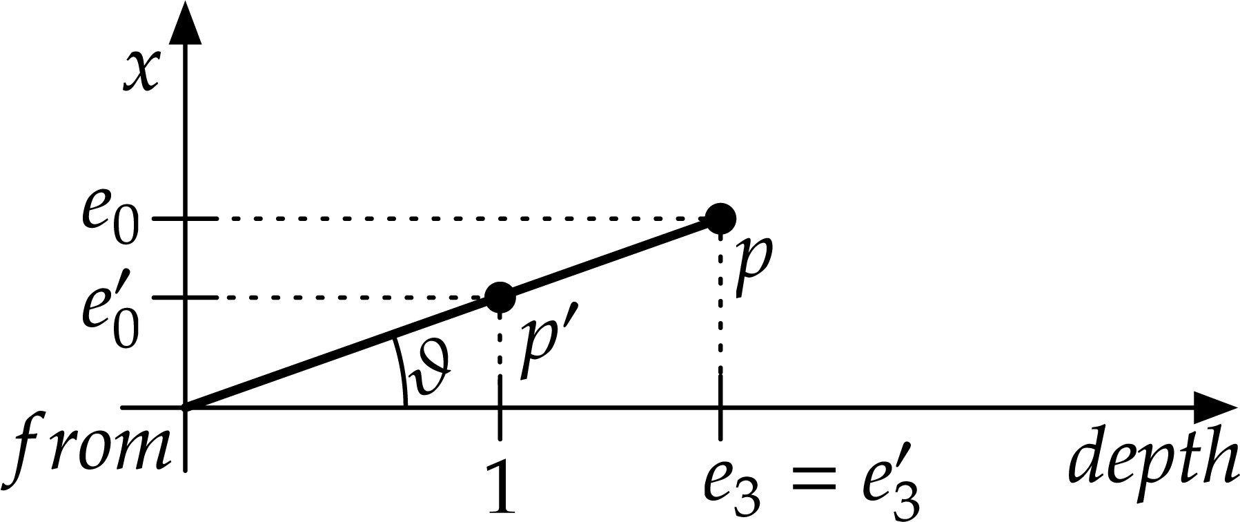
Methodology
We present here three different projections from ℝn to ℝn−1 which can be applied iteratively to bring objects of any dimension down to 3D for display. We three projections that are reasonably intuitive in 4D to 3D: a ‘long axis’ projection that puts 3D objects side by side, the orthographic and perspective projections that work in the same way as their 3D to 2D analogues, and a projection to an (n − 1)-sphere followed by a stereographic projection to ℝn−1.
‘Long axis’ projection
First we aim to replicate the idea behind the example previously shown in Fig. 1—a series of 3D objects that are shown next to each other, seemingly projected separately with the correspondences across scale or time shown as long edges (as in Fig. 1) or faces connecting the 3D objects. Edges would join correspondences between vertices across the models, while faces would join correspondences between elements of dimension up to one (e.g. a pair of edges, or an edge and a vertex). Since every 3D object is apparently projected separately using a perspective projection to 2D, it is thus shown in the same intuitive way in which a single 3D object is projected down to 2D. The result of this projection is shown in Fig. 3 for the model previously shown in Figs. 1 and in 4 for a 4D model using 3D space with time.
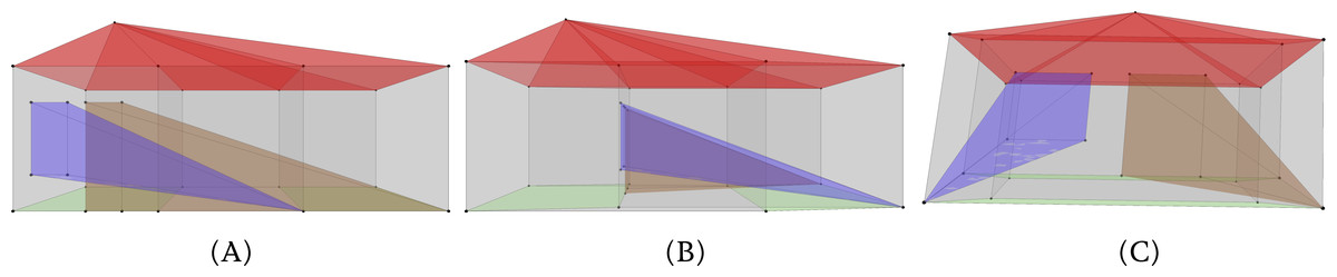
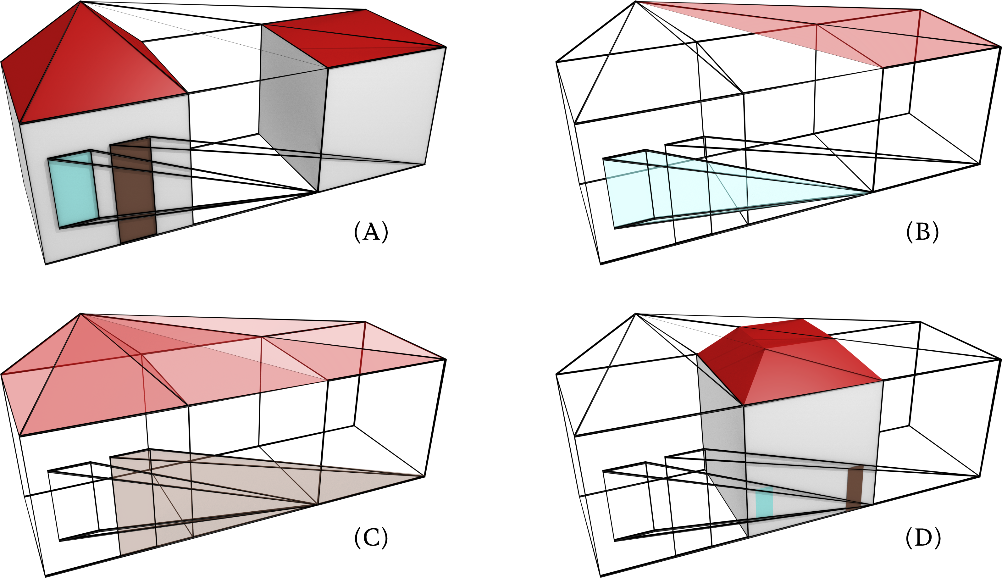
Figure 3: A model of a 4D house similar to the example shown previously in Fig. 1, here including also a window and a door that are collapsed to a vertex in the 3D object at the lower level of detail.
(A) shows the two 3D objects positioned as in Fig. 1, (B) rotates these models 90° so that the front of the house is on the right, and (C) orients the two 3D objects front to back. Many more interesting views are possible, but these show the correspondences particularly clearly. Unlike the other model, this one was generated with 4D coordinates and projected using our prototype that applies the projection described in this section.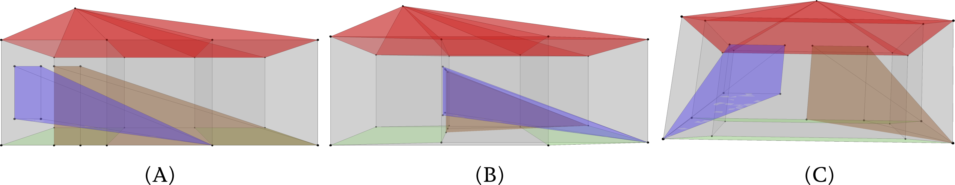
![We take (A) a simple 3D model of two buildings connected by an elevated corridor, and model it in 4D such that the two buildings exist during a time interval [ − 1, 1] and the corridor only exists during [ − 0.67, 0.67], resulting in (B) a 4D model shown here in a ‘long axis’ projection.](https://dfzljdn9uc3pi.cloudfront.net/2017/cs-123/1/fig-4-2x.jpg)
Figure 4: We take (A) a simple 3D model of two buildings connected by an elevated corridor, and model it in 4D such that the two buildings exist during a time interval [ − 1, 1] and the corridor only exists during [ − 0.67, 0.67], resulting in (B) a 4D model shown here in a ‘long axis’ projection.
The two buildings are shown in blue and green for clarity. Note how this model shows more saturated colours due to the higher number of faces that overlap in it.
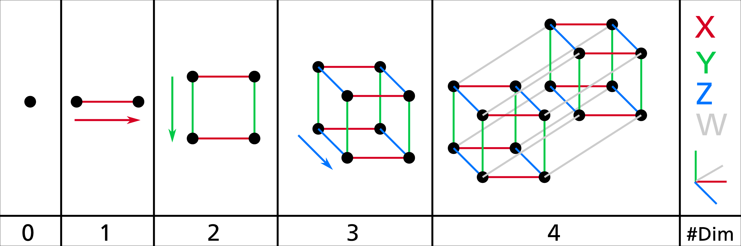
Although to the best of our knowledge this projection does not have a well-known name, it is widely used in explanations of 4D and nD geometry—especially when drawn by hand or when the intent is to focus on the connectivity between different elements. For instance, it is usually used in the typical explanation for how to construct a tesseract, i.e., a 4-cube or the 4D analogue of a 2D square or 3D cube, which is based on drawing two cubes and connecting the corresponding vertices between the two (Fig. 5). Among other examples in the scientific literature, this kind of projection can be seen in Fig. 2 in Yau & Srihari (1983), Fig. 3.4 in Hollasch (1991), Fig. 3 in Banchoff & Cervone (1992), Figs. 1–4 in Arenas & Pérez-Aguila (2006), Fig. 6 in Grasset-Simon, Damiand & Lienhardt (2006), Fig. 1 in Paul (2012) and Fig. 16 in Van Oosterom & Meijers (2014).
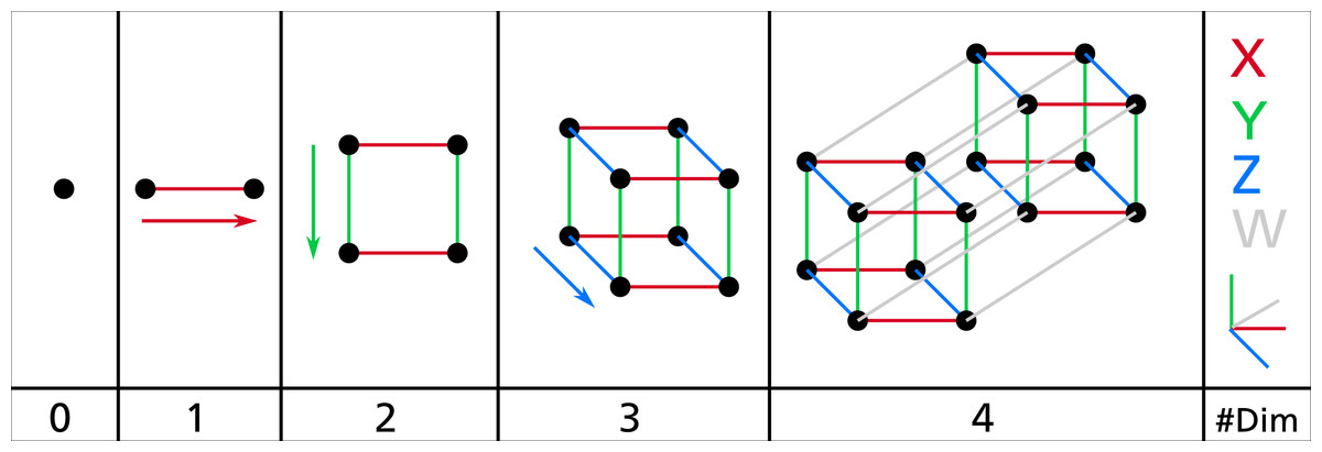
Figure 5: The typical explanation for how to draw the vertices and edges in an i-cube.
Starting from a single vertex representing a point (i.e. a 0-cube), an (i + 1)-cube can be created by drawing two i-cubes and connecting the corresponding vertices of the two. Image by Wikimedia user NerdBoy1392 (retrieved from https://commons.wikimedia.org/wiki/File:Dimension_levels.svg under a CC BY-SA 3.0 license).
Conceptually, describing this projection from n to n − 1 dimensions, which we hereafter refer to as a ‘long axis’ projection, is very simple. Considering a set of points P in ℝn, the projected set of points P′ in ℝn−1 is given by taking the coordinates of P for the first n − 1 axes and adding to them the last coordinate of P which is spread over all coordinates according to weights specified in a customisable vector . For instance, Fig. 3 uses , resulting in 3D models that are 2 units displaced for every unit in which they are apart along the n-th axis. In matrix form, this kind of projection can then be applied as .
Orthographic and perspective projections
Another reasonably intuitive pair of projections are the orthographic and perspective projections from nD to (n − 1)D. These treat all axes similarly and thus make it more difficult to see the different (n − 1)-dimensional models along the n-th axis, but they result in models that are much less deformed. Also, as shown in the 4D example in Fig. 6, it is easy to rotate models in such a way that the corresponding features are easily seen.
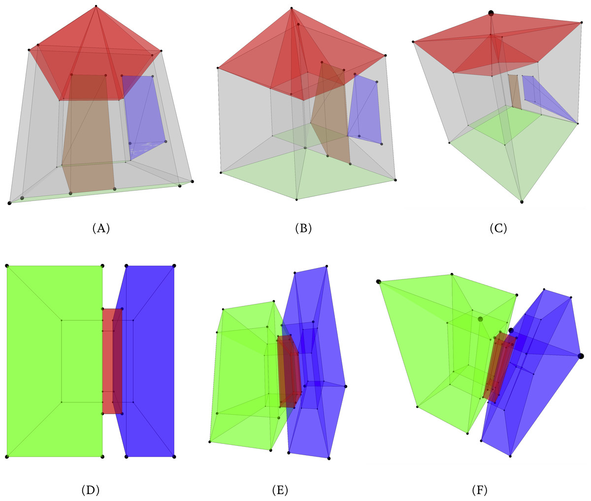
Figure 6: (A–C) The 4D house model and (D–F) the two buildings model projected down to 3D using an orthographic projection.
The different views are obtained by applying different rotations in 4D. The less and more detailed 3D models can be found by looking at where the door and window are collapsed.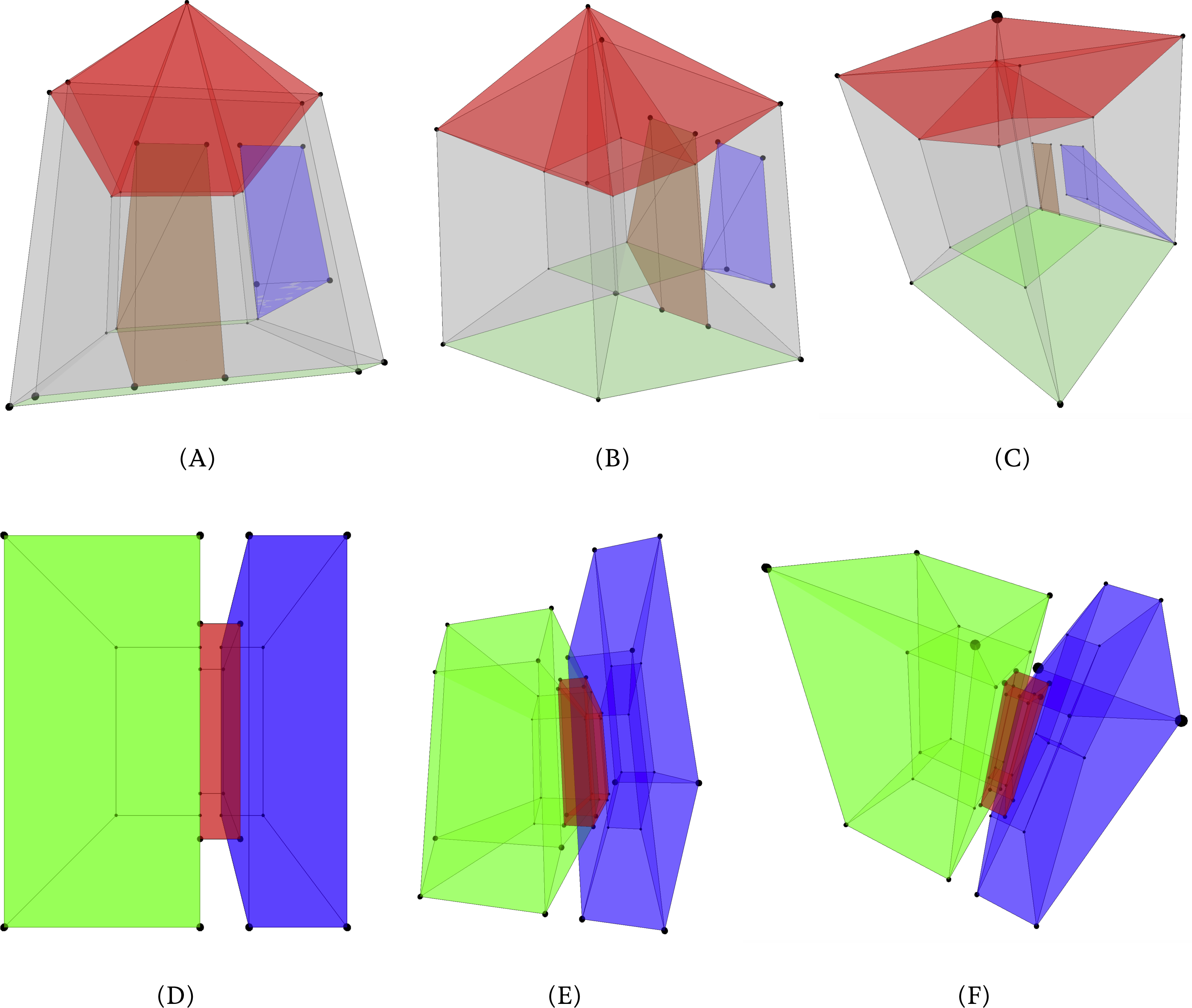
Based on the description of 4D-to-3D orthographic and perspective projection described from Hollasch (1991), we here extend the method in order to describe the n-dimensional to ( n − 1)-dimensional case, changing some aspects to give a clearer geometric meaning for each vector.
Similarly, we start with a point from ∈ ℝn where the viewer is located, a point to ∈ ℝn that the viewer directly points towards (which can be easily set to the centre or centroid of the dataset), and a set of n − 2 initial vectors in ℝn that are not all necessarily orthogonal but nevertheless are linearly independent from each other and from the vector to − from. In this setup, the vectors serve as a base to define the orientation of the system, much like the traditional vector that is used in 3D to 2D projections and the vector described previously. From the above mentioned variables and using the nD cross-product, it is possible to define a new set of orthogonal unit vectors that define the axes x0, …, xn−1 of a coordinate system in ℝn as:
The vector is the first that needs to be computed and is oriented along the line from the viewer (from) to the point that it is oriented towards (to). Afterwards, the vectors are computed in order from to as normalised n-dimensional cross products of n − 1 vectors. These contain a mixture of the input vectors and the computed unit vectors , starting from n − 2 input vectors and one unit vector for , and removing one input vector and adding the previously computed unit vector for the next vector. Note that if and are all orthogonal to each other, ∀0 < i < n − 1, is simply a normalised .
Like in the previous case, the vectors can then be used to transform an m × n matrix of mnD points in world coordinates P into an m × n matrix of mnD points in eye coordinates E by applying the following transformation:
As before, if E has rows of the form representing points, e0, …, en−2 are directly usable as the coordinates in ℝn−1 of the projected point in an n-dimensional to (n − 1)-dimensional orthographic projection, while en−1 represents the depth, i.e. the distance between the point and the projection (n − 1)-dimensional subspace, which can be used for visual cues2 . The coordinates along e0, …, en−2 could be made to fit within a certain bounding box by computing their extent along each axis, then scaling appropriately using the extent that is largest in proportion to the extent of the bounding box’s corresponding axis.
For an n-dimensional to (n − 1)-dimensional perspective projection, it is only necessary to compute the distance between a point and the viewer along every axis by taking into account the viewing angle ϑ between and the line between the to point and every point. Intuitively, this means that if an object is n times farther than another identical object, it is depicted n times smaller, or of its size. This situation is shown in Fig. 7 and results in new coordinates that are shifted inwards. The coordinates are computed as:
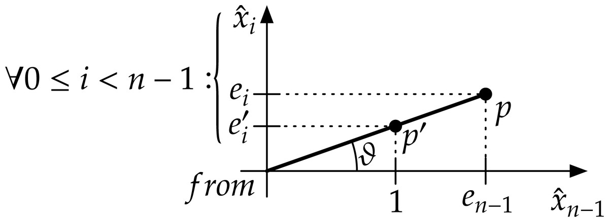
Figure 7: The geometry of an nD perspective projection for a point p.
By analysing each axis ( ∀0 ≤ i < n − 1) independently together with the final axis , it is possible to see that the coordinates of the point along that axis, given by ei, are scaled inwards based on the viewing angle ϑ.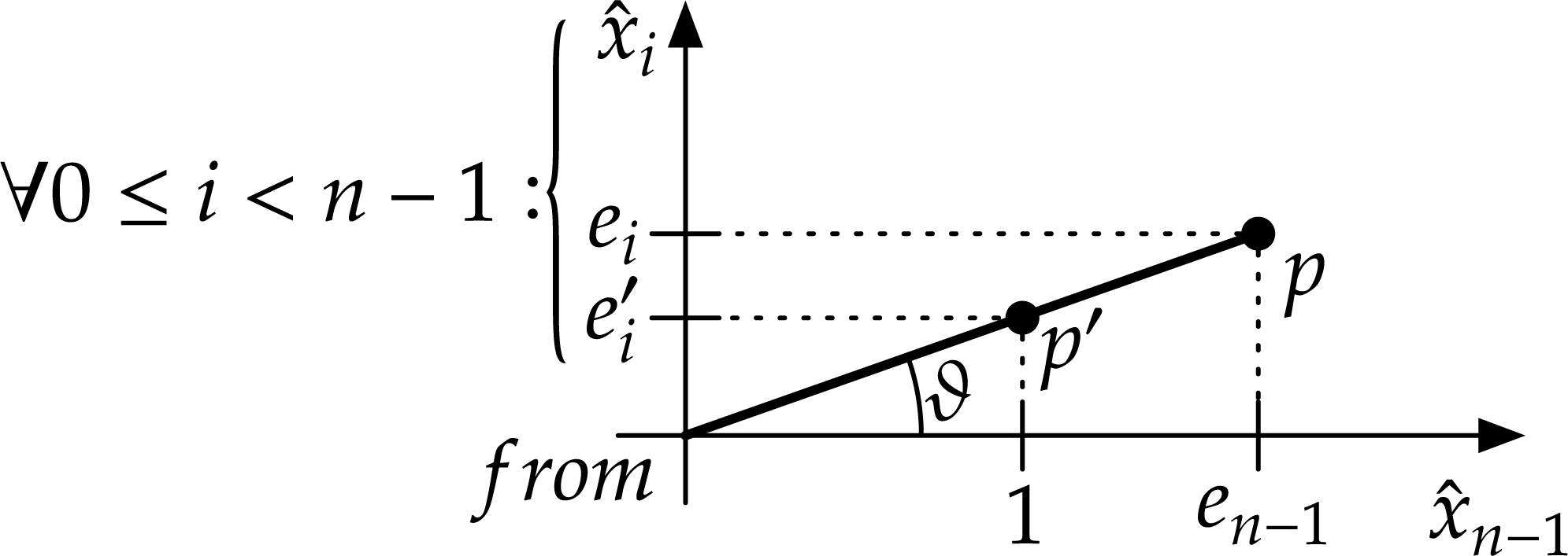
The (n − 1)-dimensional coordinates generated by this process can then be recursively projected down to progressively lower dimensions using this method. The objects represented by these coordinates can also be discretised into images of any dimension. For instance, Hanson (1994) describes how to perform many of the operations that would be required, such as dimension-independent clipping tests and ray-tracing methods.
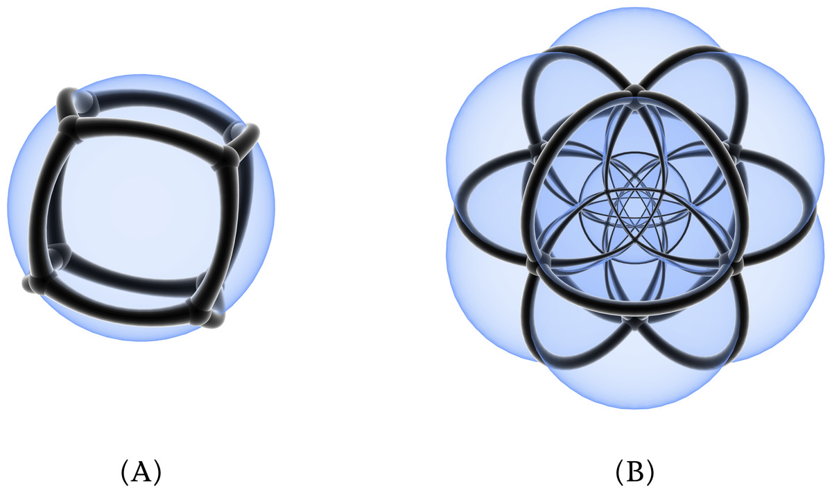
Figure 8: A polyhedron and a polychoron in Jenn 3D: (A) a cube and (B) a 24-cell.
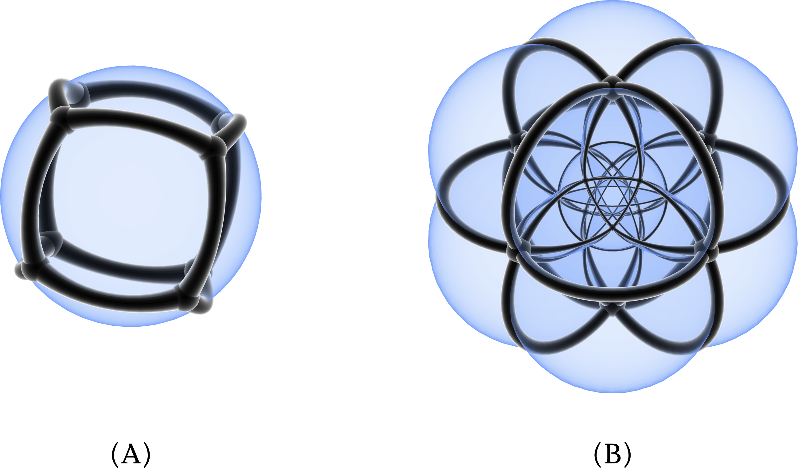
Stereographic projection
A final projection possibility is to apply a stereographic projection from ℝn to ℝn−1, which for us was partly inspired by Jenn 3D (http://www.math.cmu.edu/ fho/jenn/) (Fig. 8). This program visualises polyhedra and polychora embedded in ℝ4 by first projecting them inwards/outwards to the volume of a 3-sphere3 and then projecting them stereographically to ℝ3, resulting in curved edges, faces and volumes.
In a dimension-independent form, this type of projection can be easily done by considering the angles ϑ0, …, ϑn−2 in an n-dimensional spherical coordinate system. Steeb (2011, §12.2) formulates such a system as:
It is worth to note that the radius r of such a coordinate system is a measure of the depth with respect to the projection (n − 1)-sphere Sn−1 and can be used similarly to the previous projection examples. The points can then be converted back into points on the surface of an (n − 1)-sphere of radius 1 by making r = 1 and applying the inverse transformation. Steeb (2011, §12.2) formulates it as:
The next step, a stereographic projection, is also easy to apply in higher dimensions, mapping an (n + 1)-dimensional point x = (x0, …, xn) on an n-sphere Sn to an n-dimensional point x′ = (x0, …, xn−1) in the n-dimensional Euclidean space ℝn. Chisholm (2000) formulates this projection as:
The stereographic projection from nD to (n − 1)D is particularly intuitive because it results in the n-th axis being converted into an inwards-outwards axis. As shown in Fig. 9, when it is applied to scale, this results in models that decrease or increase in detail as one moves inwards or outwards. The case with time is similar: as one moves inwards/outwards, it is easy to see the state of a model at a time before/after.
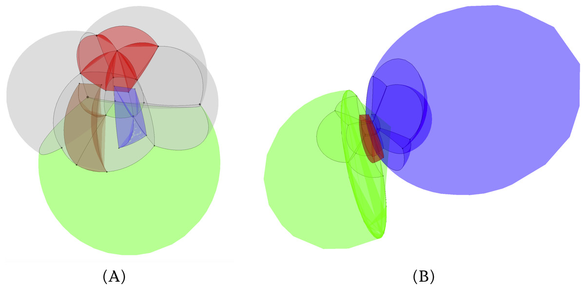
Figure 9: (A) The 4D house model and (B) the two buildings model projected first inwards/outwards to the closest point on the 3-sphere S3 and then stereographically to ℝ3.
The round surfaces are obtained by first refining every face in the 4D models.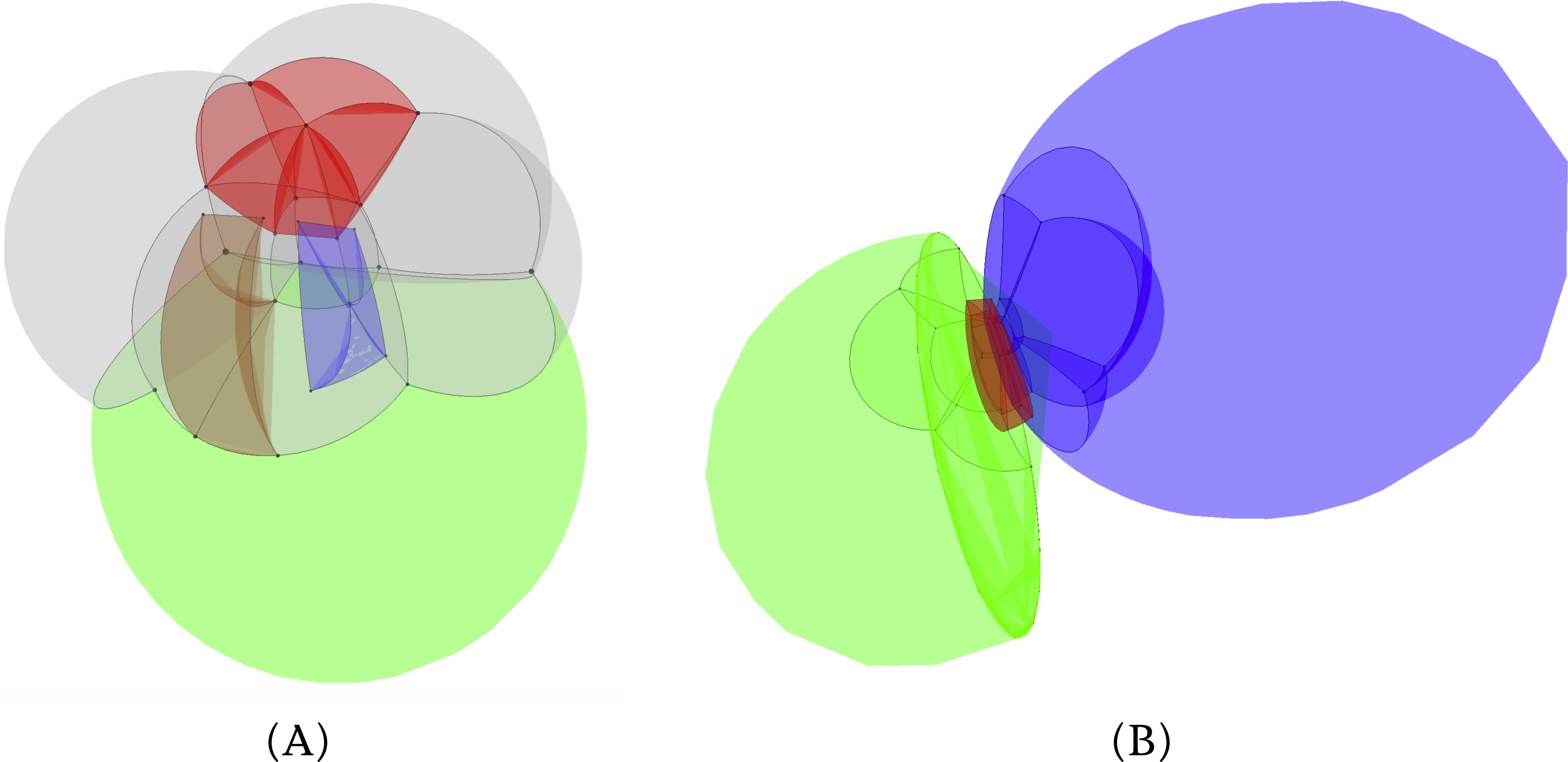
Results
We have implemented a small prototype for an interactive viewer of arbitrary 4D objects that performs the three projections previously described. It was used to generate Figs. 3, 6 and 9, which were obtained by moving around the scene, zooming in/out and capturing screenshots using the software.
The prototype was implemented using part of the codebase of azul (https://github.com/tudelft3d/azul) and is written in a combination of Swift 3 and C++11 using Metal—a low-level and low-overhead graphics API—under macOS 10.12 (https://developer.apple.com/metal/). By using Metal, we are able to project and display objects with several thousand polygons with minimal visual lag on a standard computer. Its source code is available under the GPLv3 licence at https://github.com/kenohori/azul4d.
We take advantage of the fact that the Metal Shading Language—as well as most other linear algebra libraries intended for computer graphics—has appropriate data structures for 4D geometries and linear algebra operations with vectors and matrices of size up to four. While these are normally intended for use with homogeneous coordinates in 3D space, they can be used to do various operations in 4D space with minor modifications and by reimplementing some operations.
Unfortunately, this programming trick also means that extending the current prototype to dimensions higher than four requires additional work and rather cumbersome programming. However, implementing these operations in a dimension-independent way is rather not difficult outside in a more flexible programming environment. For instance, Fig. 10 shows how a double stereographic projection can be used to reduce the dimensionality of an object from 5D to 3D. This figure was generated in a separate C+ + program which exports its results to an OBJ file. The models were afterwards rendered in Blender (https://www.blender.org).
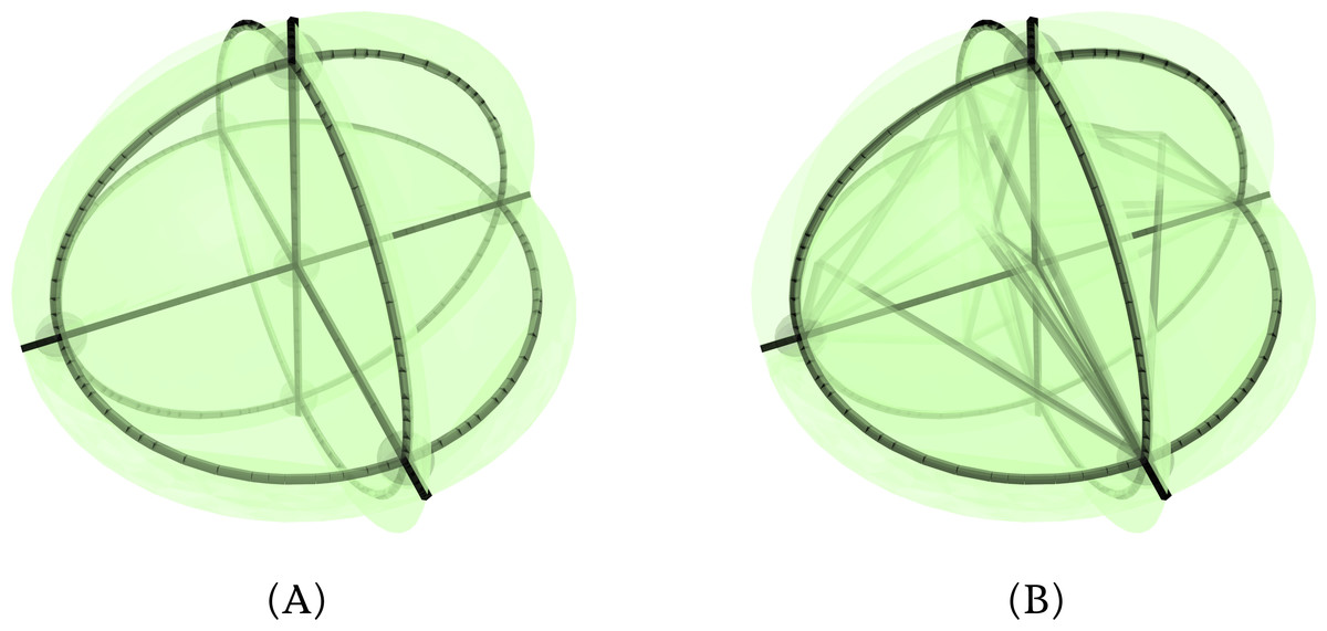
Figure 10: (A) A stereographic projection of a 4-orthoplex and (B) a double stereographic projection of a 5-orthoplex.
The family of orthoplexes contains the analogue shapes of a 2D square or a 3D octahedron.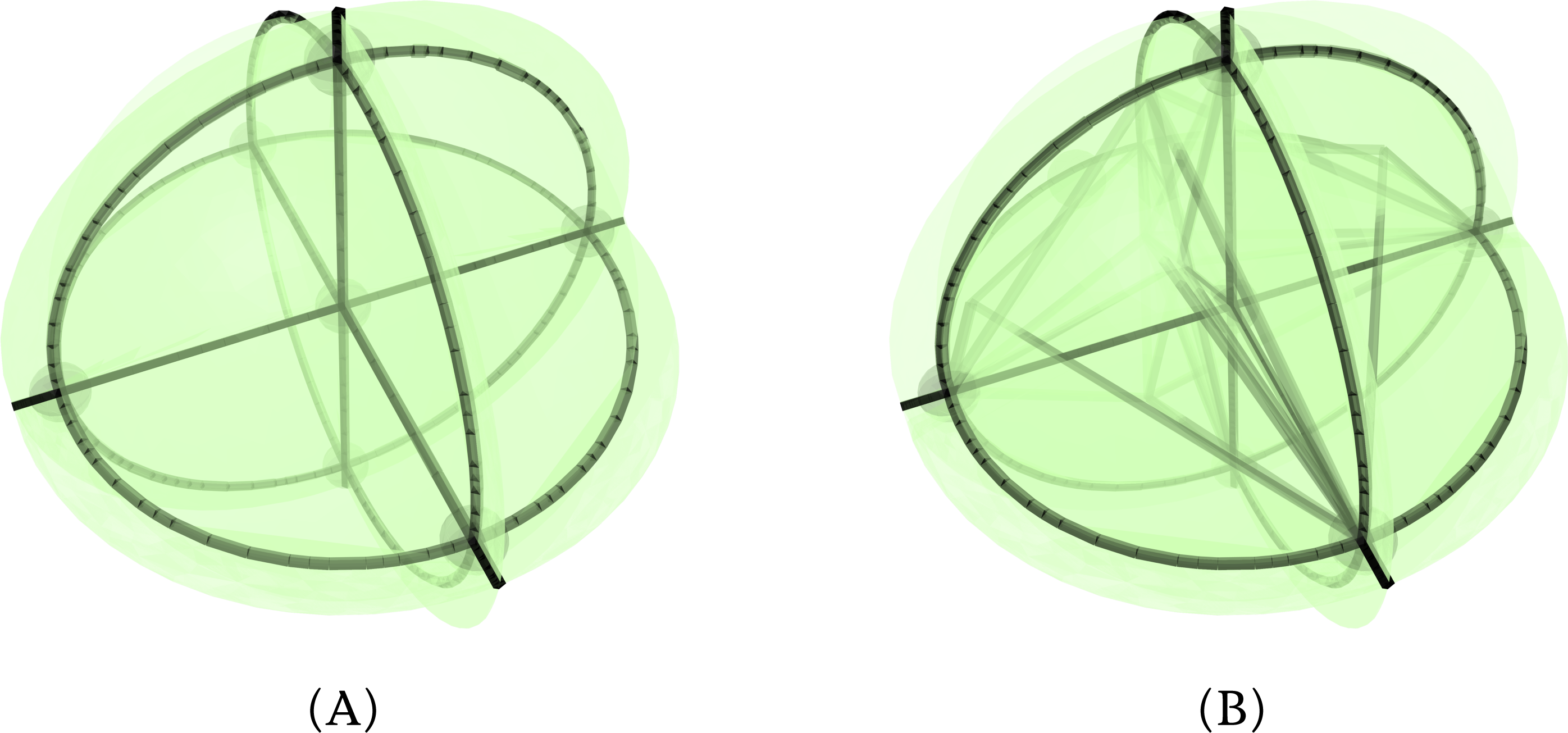
In our prototype, we only consider the vertices, edges and faces of the 4D objects, as the higher-dimensional 3D and 4D primitives—whose 0D, 1D and 2D boundaries are however shown—would readily obscure each other in any sort of 2D or 3D visualisation (Banks, 1992). Every face of an object is thus stored as a sequence of vertices with coordinates in ℝ4 and is appended with an RGBA colour attribute with possible transparency. The alpha value of each face is used see all faces at once, as they would otherwise overlap with each other on the screen.
The 4D models were manually constructed based on defining their vertices with 4D coordinates and their faces as successions of vertices. In addition to the 4D house previously shown, we built a simpler tesseract for testing. As built, the tesseract consists of 16 vertices and 24 vertices, while the 4D house consists of 24 vertices and 43 faces. However, we used the face refining process described below to test our prototype with models with up to a few thousand faces. Once created, the models were still displayed and manipulated smoothly.
To start, we preprocess a 4D model by triangulating and possibly refining each face, which makes it possible to display concave faces and to properly see the curved shapes that are caused by the stereographic projection previously described. For this, we first compute the plane passing through the first three points of each face4 and project each point from ℝ4 to a new coordinate system in ℝ2 on the plane. We then triangulate and refine separately each face in ℝ2 with the help of a few packages of the Computational Geometry Algorithms Library (CGAL) (http://www.cgal.org), and then we reproject the results back to the previously computed plane in ℝ4.
We then use a Metal Shading Language compute shader—a technique to perform general-purpose computing on graphics processing units (GPGPU)—in order to apply the desired projection from ℝ4 to ℝ3. The three different projections presented previously are each implemented as a compute shader. By doing so, it is easier to run them as separate computations outside the graphics pipeline, to then extract the projected ℝ3 vertex coordinates of every face and use them to generate separate representations of their bounding edges and vertices5 . Using their projected coordinates in ℝ3, the edges and vertices surrounding each face are thus displayed respectively as possibly refined line segments and as icosahedral approximations of spheres (i.e., icospheres).
Finally, we use a standard perspective projection in a Metal vertex shader to display the projected model with all its faces, edges and vertices. We use a couple of tricks in order to keep the process fast and as parallel as possible: separate threads for each CPU process (the generation of the vertex and edge geometries and the modification of the projection matrices according to user interaction) and GPU process (4D-to-3D projection and 3D-to-2D projection for display), and blending with order-independent transparency without depth checks. For complex models, this results in a small lag where the vertices and edges move slightly after the faces.
In the current prototype, we have implemented a couple functions to interact with the model: rotations in 4D and translations in 3D. In 4D, the user can rotate the model around the six possible rotation planes by clicking and dragging while pressing different modifier keys. In 3D, it is possible to move a model around using 2D scrolling on a touchpad to shift it left/right/up/down and using pinch gestures to shift it backward/forward (according to the current view).
Discussion and Conclusions
Visualising complete 4D and nD objects projected to 3D and displayed in 2D is often unintuitive, but it enables analysing higher-dimensional objects in a thorough manner that cross-sections do not. The three projections we have shown here are nevertheless reasonably intuitive due to their similarity to common projections from 3D to 2D, the relatively small distortions in the models and the existence of a clear fourth axis. They also have a dimension-independent formulation.
There are however many other types of interesting projections that can be defined in any dimension, such as the equirectangular projection where evenly spaced angles along a rotation plane can be directly converted into evenly spaced coordinates—in this case covering 180°vertically and 360°horizontally. Extending such a projection to nD would result in an n-orthotope, such as a (filled) rectangle in 2D or a cuboid (i.e., a box) in 3D.
By applying the projections shown in this paper to 4D objects depicting 3D objects that change in time or scale, it is possible to see at once all correspondences between different elements of the 3D objects and the topological relationships between them.
Compared to other 4D visualisation techniques, we opt for a rather minimal approach without lighting and shading. In our application, we believe that this is optimal due to better performance and because it makes for simpler-looking and more intuitive output. In this manner, progressively darker shades of a colour are a good visual cue for the number of faces of the same colour that are visually overlapping at any given point. Since we apply the projection from 4D to 3D in the GPU, it is not efficient to extract the surfaces again in order to compute the 3D normals required for lighting in 3D, while lighting in 4D results in unintuitive visual cues.