
Intelligent control strategy for industrial furnaces based on yield classification prediction using a gray relative correlation-convolutional neural network-multilayer perceptron (GCM) machine learning model
- Published
- Accepted
- Received
- Academic Editor
- Ivan Miguel Pires
- Subject Areas
- Algorithms and Analysis of Algorithms, Artificial Intelligence, Data Mining and Machine Learning, Scientific Computing and Simulation, Neural Networks
- Keywords
- Yield classification prediction, Machine learning, Intelligent control strategy, Industrial furnace
- Copyright
- © 2024 Guo et al.
- Licence
- This is an open access article distributed under the terms of the Creative Commons Attribution License, which permits unrestricted use, distribution, reproduction and adaptation in any medium and for any purpose provided that it is properly attributed. For attribution, the original author(s), title, publication source (PeerJ Computer Science) and either DOI or URL of the article must be cited.
- Cite this article
- 2024. Intelligent control strategy for industrial furnaces based on yield classification prediction using a gray relative correlation-convolutional neural network-multilayer perceptron (GCM) machine learning model. PeerJ Computer Science 10:e1836 https://doi.org/10.7717/peerj-cs.1836
Abstract
Industrial furnaces still play an important role in national economic growth. Owing to the complexity of the production process, the product yield fluctuates, and cannot be executed in real time, which has not kept pace with the development of the intelligent technologies in Industry 4.0. In this study, based on the deep learning theory and operational data collected from more than one year of actual production of a lime kiln, we proposed a hybrid deep network model combining a gray relative correlation, a convolutional neural network and a multilayer perceptron model (GCM) to categorize production processes and predict yield classifications. The results show that the loss and calculation time of the model based on the screened set of variables are significantly reduced, and the accuracy is almost unaffected; the GCM model has the best performance in predicting the yield classification of lime kilns. The intelligent control strategy for non-fault state is then set according to the predicted yield classification. Operating parameters are adjusted in a timely manner according to different priority control sequences to achieve higher yield, ensure high production efficiency, reduce unnecessary waste, and save energy.
Introduction
With the emerging Industry 4.0 revolution, traditional manufacturing is facing the reality that it is going to have to transform. One of the key reforms inherent in Industry 4.0 is the use of intelligent technology for intelligent decision making. This is also the traditional manufacturing industry, especially the high energy consumption industry in urgent need of development direction. Among them, industrial furnaces are relatively typical industries with high energy consumption and relatively low intelligence level. Industrial furnaces are large energy consumers in China, with the total number reaching more than 200,000 sets, among which fuel furnaces account for 55% of the total number and 92% of energy consumption, which is 23% of the country’s energy consumption (Chen, Wang & Sun, 2017). The traditional industrial furnace has high energy consumption, low benefits, significant waste of resources, and environmental pollution, which is inconsistent with the goals of energy conservation and emission reduction, at the same time, it is not in line with the development of the inherent needs of Industry 4.0 for intelligent technology.
As traditional industrial furnaces have reached their thermodynamic limits (Lüngen & Schmöle, 2004), other novel or disruptive technologies are needed. Common energy conservation measures are based on improving the efficiency of equipment, such as oxygen blast furnace (Arasto et al., 2014), the flue gas recirculation and supplementary burnout air (Yan et al., 2021), “treating waste with waste” strategy for desulfurization using electric arc furnace dust (Jia et al., 2023). In addition, energy conservation measures based on software improvements such as control methods exist (Obika & Yamamoto, 2018). A series of studies have emerged in stable equipment owing to a safe operating environment, good control effects, high return on investment, and easy implementation. Bakdi, Kouadri & Bensmail (2017) features an adaptive threshold monitoring schemethat uses principal component analysis to diagnose faults in cement rotary kilns. Yu et al. (2018) developed a multiobjective operational model using a teaching-learning-based optimization algorithm for an industrial cracking furnace system, resulting in higher product yields and lower fuel consumption. A soft sensor model for estimating the rotor deformation of air preheaters in a thermal power plant boiler is studied, based on a deep learning network combining stacked auto-encoders with support vector regression (Wang & Liu, 2018). An Internet of Things-enabled model-based approach was proposed, including a parameter optimization model and energy-aware incident control strategy (Liu et al., 2020). Wang et al. (2022a) and Wang et al. (2022b) proposed a novel attention-based dynamic stacked autoencoder networks for soft sensor modeling to reflect the dynamic historical data information of the production status under irregular sampling frequency. Wang et al. (2022a) and Wang et al. (2022b) proposed the multi-label transfer reinforcement learning (ML-TRL) methods to recognize the compound fault. Song & Liu (2023) combined a pseudo-Siamese network (PSN) and robust model aggregation to propose a federated domain generalization approach for intelligent fault diagnosis. Li et al. (2023) proposed a deep continual transfer learning network with dynamic weight aggregation which can effectively handle the industrial streaming data under different working conditions.
Currently, a part of the control system utilizes an operation optimization and control algorithm that has self-adaptive, self-learning, and automatic adjustment capabilities. However, it cannot adequately adapt to dynamic changes in industrial processes, leading to poor control performance. In particular, industrial processes such as calcination furnaces are characterized by different time scales, strong nonlinearity, multivariate strong coupling, unclear mechanisms, and impossible real-time online measurement of yield and quality. Therefore, the feedback control, operation index target-value range decision, and abnormal operation condition diagnosis and treatment of the system are mostly performed by technical personnel and experts. This type of industrial process is often in a non-optimal operation state.
In this study, based on the deep learning theory and more than one year of actual production operational data, we established a gray relative correlation-convolutional neural network-multilayer perceptron (GCM) model to predict the yield classification of a sleeve kiln with thermal cycle. Firstly, we use the gray relative correlation degree to calculate the correlation degree between variables and yield, and select the variables with a higher correlation degree for model calculation. Then, the preprocessed datasets are fed into a hybrid deep network model based on the convolutional neural network (CNN) and multilayer perceptron (MLP) networks to predict yield classifications. We conducted extensive experiments using five methods on industrial datasets for multiple classification forecasting to compare the performance of the CNN-MLP model. An Intelligent control strategy for non-fault state is proposed according to different yield classification. Finally, by calculating the actual production data fo a lime kiln, the increase of yield is obvious. Predicting the yield classification by the current main state variables can provide technicians with intuitive and fast prediction results so that technicians or control systems can adjust the production process in a timely manner to ensure high production efficiency, reduce unnecessary waste, and save energy.
The remainder of this study is organized as follows: ‘Research Background and Process Description’ describes the technological process of lime kilns with thermal cycle and formulates the problem. ‘Modeling Methodology’ describes the data preparation method and the structure of the gray relative correlation-convolutional neural network-multilayer perceptron (GCM) model used to predict the yield classifications. ‘Experiments and discussion’ illustrates the experimental results, and the Intelligent control strategy for non-fault state is proposed. Then, the increased yield is estimated. Finally, ‘Conclusion’ concludes the article.
Research Background and Process Description
Research background
With the rise of the Industry 4.0 revolution, the development of modern computer technology, including artificial intelligence, has made it urgent to establish a technical foundation for intelligent control to improve the automatic control quality and energy conservation in large-scale complex system control. As a result, academia and industry are conducting extensive research on intelligent algorithms and data-driven prediction models. In particular, several studies have emerged in the field of industry furnace.
Among these studies, research on predicting temperature is relatively common. Su et al. (2019) used adaptive particle swarm optimization (APSO) to improve the prediction accuracy and generalization performance of a multi-layer extreme learning machine model to predict the hot metal temperature in the blast furnace. Zhang et al. (2019) proposed an ensemble random vector functional link network for shuttle kiln temperature prediction, while Leon-Medina et al. (2021) used a GRU layer and dense layer to predict temperature in a 75 MW electric arc furnace for ferronickel production. Zhang et al. (2021) proposed a hybrid deep network model for sintering temperature forecasting in a rotary kiln.
Other common research includes the prediction of the component content. Jiang et al. (2019) proposed a sintering parameter identification model using a nonlinear autoregressive model with exogenous input (NARX) algorithm. Pham, Ridley & Lazarescu (2020) presented a material ring detection system in alumina rotary kilns using a feature extraction method, achieving an accuracy of approximately 96%. Zhou et al. (2020) developed an improved gated recurrent unit-recurrent neural network (GRU-RNN) for predicting hot metal silicon content with a 92.4% hit rate.
Some studies have also focused on predicting various states. Wang, Song & Chen (2017) used deep neural network (DNN) and convolutional neural network (CNN) to predict combustion state and heat release rate. Kim et al. (2019) developed a multivariate time-series forecasting algorithm using CNN and long short-term memory (LSTM) to predict blast furnace opening and closing times with over 90% accuracy. Chen et al. (2020) established a Time-Between-Failure (TBF) prediction model through a data-driven approach based proportional hazard deep learning. And a long-short-term memory (LSTM) network was established to train the TBF prediction model based on the pre-processed maintenance data. To develop an more excellent quality prediction model for coal preparation process, Yin et al. (2021) proposed a semi-supervised soft sensor modeling approach combining Stacked Auto-Encoder with Bidirectional Long Short-Term Memory. Lee, Bae & Kim (2021) proposed an uncertainty-aware soft sensor that uses Bayesian recurrent neural networks (RNNs) to increase the reliability of predictive uncertainty. Miao et al. (2022) used a genetic algorithm to evaluate the environmental impact of turbine-integrated steam methane reforming. Heat load in blast furnace was predicted based CNN combined with a bidirectional long short-term memory network (Xu et al., 2023).
Using intelligent algorithms and computer programs can optimize equipment operation to improve product output and quality while reducing energy consumption. The integration of algorithms is a trend in process control, optimization, fault diagnosis, and self-healing control in the furnace industry. However, most furnace prediction results require expert interpretation, causing time lag problems that affect yield, quality, and timely loss prevention and energy consumption reduction.
Process description
This study focuses on a sleeve kiln with a thermal cycle, shown in Fig. 1. Material enters from the top, passes through preheating, calcination, and cooling zones, and is discharged from the bottom. Cooling air enters through the ash hole, flows upward, and exits through the air duct above the upper fire box. The gas exits in two parts, with part discharged from the chimney and the other entering the heat exchanger to transfer heat to ejection air. Cooled air is supplied to the lower inner cylinder by a fan, and to the upper inner cylinder through the top air pipe. Lower distribution pipe collects cooled air and distributes it to the burner. Air is preheated to around 150 °C when it flows through the lower inner collet wall.
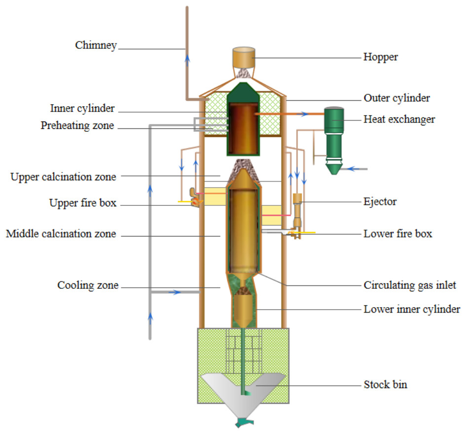
Figure 1: Structure of sleeve kiln with thermal cycle.
After the gas is introduced into the main gas pipeline in the kiln area, it is preheated and transported through the gas pipeline to the lower part of the kiln body’s gas ring. It is then divided into upper and lower combustion chamber gas branches, which are extracted from the gas ring. There are six burners on both the upper and lower parts of the kiln body, and each burner corresponds to a temperature detection device inside the combustion chamber to monitor the temperature. Other parameters such as flow rate, pressure, temperature, etc., are collected by corresponding sensors and transmitted, displayed, and stored using the existing DCS system of the enterprise. This article directly adopts the operation parameters of the production process of the enterprise.
In addition to the calcination system, other six subsystems include: flue gas system, exhaust gas system, thermal cycle system, cooling system, dust pelletizing system and discharge system. The main operating parameters involved in each subsystem are shown in Table 1.
| Classification | Operating parameters |
|---|---|
| Calcination system | Upper arch bridge temperature, Lower arch bridge temperature, Lower combustor temperature, Setting temperature of upper combustor, Bottom temperature of upper inner cylinder, Negative pressure of lower combustor |
| Flue gas system | Gas flow rate of upper combustor, Gas flow rate of lower combustor, Gas flow, Downstream pressure for quick breaking valve of gas header pipe, Calorific value of gas, Inlet and outlet pressure of gas booster fan |
| Exhaust gas system | Exhaust gas temperature at kiln top, Fan frequency and electric current for High-temperature exhaust gas |
| Thermal cycle system | Circulating gas temperature, Drive air loop temperature, Outlet and inlet temperatures of heat exchanger exhaust gas, Mixing temperature of exhaust gas, Driving fan flow, Pressure, Frequency |
| Cooling system | Ring pipe temperature of cooling air , Upper cold flow rate, Lower cold flow rate, Air flow rate for cooling lime |
| Dust pelletizing system | Dust removal fan pressure, Differential pressure, Dust removal temperature (inlet) |
| Discharge system | Average temperature of ash discharge, Winch current, Yield, Hydraumatic oil temperature |
The manufacturing process is complex, with many variables to monitor. Three prominent characteristics of the production process are as follows:
Dynamic nonlinearity: The production process involves complex physical and chemical reactions, heat and mass transfer, multiphase fluid flow, and secondary reactions during calcination that are difficult to accurately represent in mathematical models.
Multivariate coupling: During calcination in a sleeve kiln, there are a series of variables that affect and interact with each other. Finally, all variables affect the output.
Large time lag: The calcination process takes several hours, making it difficult to know immediately whether the monitored state variables can ensure optimal yield. Furthermore, the product is the cumulative response of all variables over time.
In this study, we developed a yield classification prediction model, GCM, using production process parameters in a lime kiln. We used gray relative correlation to identify the relevant process parameters and used them to determine the input variables for a deep network model that combines CNN and MLP to predict yield classification. Based on this model, a Intelligent control strategy for non-fault state was established, with different control priorities and sequences for different yield operating classes. The technical staff can adjust the production parameters according to the control sequence to optimize yield, reduce waste and costs, and improve energy utilization and kiln production benefit.
Modeling Methodology
The prediction model based on GCM for yield classification is shown in Fig. 2. We first used gray relative correlation degree to select input variables with high correlation to yield, to improve calculation speed and reduce costs. Then, we fed the normalized input variables into the CNN-MLP Net for feature extraction and used sparse categorical cross entropy function as a loss function for yield classification prediction. The model effectively captures characteristic information through its three-part structure.
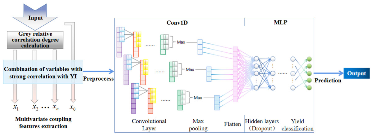
Figure 2: Algorithm framework based on the GCM model.
Gray relative correlation degree calculation
To reduce the number and cost of calculations, it is necessary to analyze the system factors. There are many systematic analysis methods in mathematical statistics, such as regression, variance, and principal component analyses. However, gray correlation analysis method is applicable to samples with or without obvious rules, and there is usually no discrepancy between the quantitative and qualitative analysis results (Wei & Gang, 2011).
The gray relative correlation degree is calculated as follows (Liu, 2017):
Assuming that X0 = (x0(1), x0(2), …, x0(n)) is system characteristic behavior sequence and is the sequence of related factors.
If the initial value image is defined as: (1) The calculation of the initial zero image of is carried out as follows: (2) Further, the gray relative correlation degree r0i is computed as follows: (3) where
Convolutional neural network and multilayer perceptron
A CNN is a structure that combines artificial neural networks and deep learning that performs well on large-scale datasets (Chen et al., 2018). The main structure of a CNN includes input, convolutional, pooling, fully connected, and output layers.
The main function of the convolutional layer is to extract features of the input data. The convolution result sequence c(n) is defined as follows: (4) where f(m) is the preprocessed input feature dataset, g(m) is the convolution kernel, len(f(m)) + len(g(m)) − 1, N is the length of f(m).
The activation function used the ReLU function (Gamarnik, Kzldag & Zadik, 2022): (5) Pooling can reduce the dimensions of the input object so that the model can extract more extensive features. Simultaneously, the input size of the next layer is reduced to reduce computation. Pooling also prevents overfitting to a certain extent (Boureau, Ponce & Lecun, 2010).
Assuming that the pooling kernel of l layer is denoted by pl ∈ ℝH×Dl, the maximum pooling result is (6) where
MLP is a forward structure artificial neural network. An MLP is made up of multiple node layers, where each layer is fully connected to the next. It has an input layer, output layer, and one or more hidden layers.
Assuming that the input layer is represented by vector I, the output of the hidden layer is (7) where W1 is the weight, b1 is the bias, f is the ReLU function.
Finally, the output layer exists. Going from the hidden layer to the output layer is a multicategory logistic regression, using softmax regression, as expressed below: (8) where k represents the index of the output neuron being computed, d is the index of all neurons in the group, and the variable z represents an array of output neurons.
Therefore, the result of the output layer is softmax(W2I1 + b2), where I1 represents the output of the hidden layer, f(W1I + b1).
Objective function and optimization strategy
Sparse categorical cross entropy was adopted in model training to measure the model prediction effectiveness. This function is computed as follows: (9) where the real label of the ith sample is , predictive value is , n is the number of predicted target classes (Integer codes, such as 1, 2, or 3......).
The adaptive moment estimation (Adam) algorithm was used to optimize the network. Adam algorithm assimilates the advantages of both the Adaptive Gradient Algorithm (Adagrad) and the Momentum-based Gradient Descent Algorithm. It utilizes momentum to accelerate convergence and automatically adjusts the learning rate decay, effectively addressing sparse gradient issues and mitigating gradient oscillation problems. Due to bias correction, the learning rate for each iteration falls within a defined range, contributing to relatively stable parameter updates. We employ the Adaptive Moment Estimation (Adam) algorithm as the gradient descent optimization method for the network.
The callback function that reduces LR on the plateau was used to optimize training. It adjusts the learning rate based on the validation set error measurement to achieve dynamic reduction. The value monitored was val_loss, and scaling was triggered when model performance did not improve after epochs of patience.
GCM model algorithm flow
The gray relative correlation degree is first used to analyze variables with high correlation to yield, allowing the variable sequence for modeling to be determined while ignoring variables with low correlation. This approach increases the efficiency of subsequent feature extraction, reduces the computational load, and improves the speed of calculation and prediction.
The data undergoes normalization and standardization processes. Due to the variety of sample attributes and their varying magnitudes, direct model learning using raw values may not be very effective. Therefore, data preprocessing becomes necessary. Based on the characteristics of the original data, the data are normalized to [0,1] by comparing them with the maximum values of the feature columns. The geometric implication of centering is that thethe centroid of the sample point cloud is aligned with the origin, resulting in an offset of the centroid of the sample point cloud. This makes the classification hyperplane closer to the origin, making the model easier to interpret.
Since the variable data corresponding to different classifications of lime yield have strong similarity and cross phenomenon, the recognition ability and anti-interference ability of the model are required to be higher when extracting characteristic information. While one of the key features of convolutional operations is the ability to enhance the original input features while reducing noise. Then, it proceeds to the convolutional layers. The convolutional layer is used in this article to perform a transformation on the input data sequence after the gray relative association screening, thereby facilitating the extraction of essential feature information from the input data. The same convolutional kernel is applied to each element of the input matrix, ensuring that only one parameter set is learned in convolutional operations, avoiding separate parameter sets for each element of the same input matrix. This significantly reduces the memory footprint of the model. The parameter sharing property of convolutional layers provides translation invariance to the network. In this article, the motion step of the convolutional kernel is set to 1.
From the perspective of the input dataset for yield classification prediction, the yield categories aren’t concentrated in a small range. When the Sigmoid function is used to propagate the gradients, it can easily filter out some important features. In normal operating data, typical values are ≥0. When values <0 appear, it indicates a malfunction, which is consistent with the pattern that the ReLU function filters. Moreover, the ReLU function has a clear advantage in its simplicity of computation. Not only is it straightforward in forward propagation, but its derivative is also simple (derivative is 1 or 0). Therefore, within the positive interval range, the vanishing gradient problem is effectively mitigated. This makes it possible to train deep networks directly in a supervised manner and has relatively faster computational speed.
After extracting features through convolutional operations, if all the resulting convolutional features are used as input for the subsequent classification, the computational load for classification will be substantial, which could lead to overfitting. Employing pooling layers has several advantages: no parameters need to be learned, the number of channels remains unchanged between input and output data after pooling, and pooling exhibits is robust to minor deviations in input features. Max pooling also maintains translational invariance within the dataset. Hence, using max pooling is a reasonable approach. Finally, the features extracted by MLP are classified to further strengthen the stability of the model and reduce the loss.
The loss function primarily measures the solution accuracy of the model, where the deviation between the model result and the actual value is proportional to the loss value. The optimization objective function is the average of the sum of the loss function values obtained from each sample. As the target labels of this dataset have been preprocessed for yield classification prior to model computation, resulting in sparse labels, the Sparse categorical cross entropy function is employed during model training to measure the model’s predictive performance. Similar to categorical cross-entropy, the former accepts sparse labels and is suitable for predicting sparse target values.
The outline of the GCM model for predicting the yield classifications in lime kiln with thermal cycle is shown in Table 2.
| Input: system characteristic behavior sequence X0 = (X0(1), X0(2), ..., X0(n)) |
| Output: yield classification |
| Gray relative correlation degree calculation: Selecting the variable array r0i with high correlation degree with yield using Eqs. (1)–(3). |
| Repeat: |
| Step1.: Preprocess data sets |
| Normalize MinMaxScaler (feature range= [0,1]), |
| add dimension on the third dimension, |
| divide the training set and test set. |
| Step2.: Convolutional Layer (CNN) |
| The first layer: Conv1D (the first time) using Eq. (4), Conv1D (the second time) using Eq. (4); MaxPooling using Eq. (6); ReLU function is an activation function obtained by Eq. (5); |
| The second and third layers: The structure is the same as that of the first layer, but the dimensions of the input data are different; |
| Flatten. |
| Step3.: Multi-layer perception (MLP) |
| A total of three hidden layers, using Eq. (7), Dropout |
| Step4.: Output layer |
| Use Eq. (8) as activation function to calculate yield classification |
| Step5.: Define training style and calculate the Loss introduced in Eq. (9); |
| Loss function using sparse_categorical_cross entropy, optimizer for computing gradients using Adam. |
| Until: If Loss <min_lr = 0.001 |
| End. |
| The callback function:Reduce LR On Plateau. Monitor is ‘val_loss’. |
Experiments and Discussion
Experimental data
Data collected in this study are the actual production data of the sleeve lime kilns from the Jie Neng Company of the Yi * Group in China. The scene of the kiln is shown in Fig. 3. The data were collected from 12 May, 2019 to 25 July, 2020, hourly each day, with a total of 57 variables. By calculating the gray relative correlation degree between production parameters, the relative correlation between each pair of parameters is obtained. The results of production parameters with a relative correlation degree greater than 50% in terms of yield are listed in Table 3. It is generally understood that when the relative correlation degree exceeds 70%, it indicates a stronger correlation.
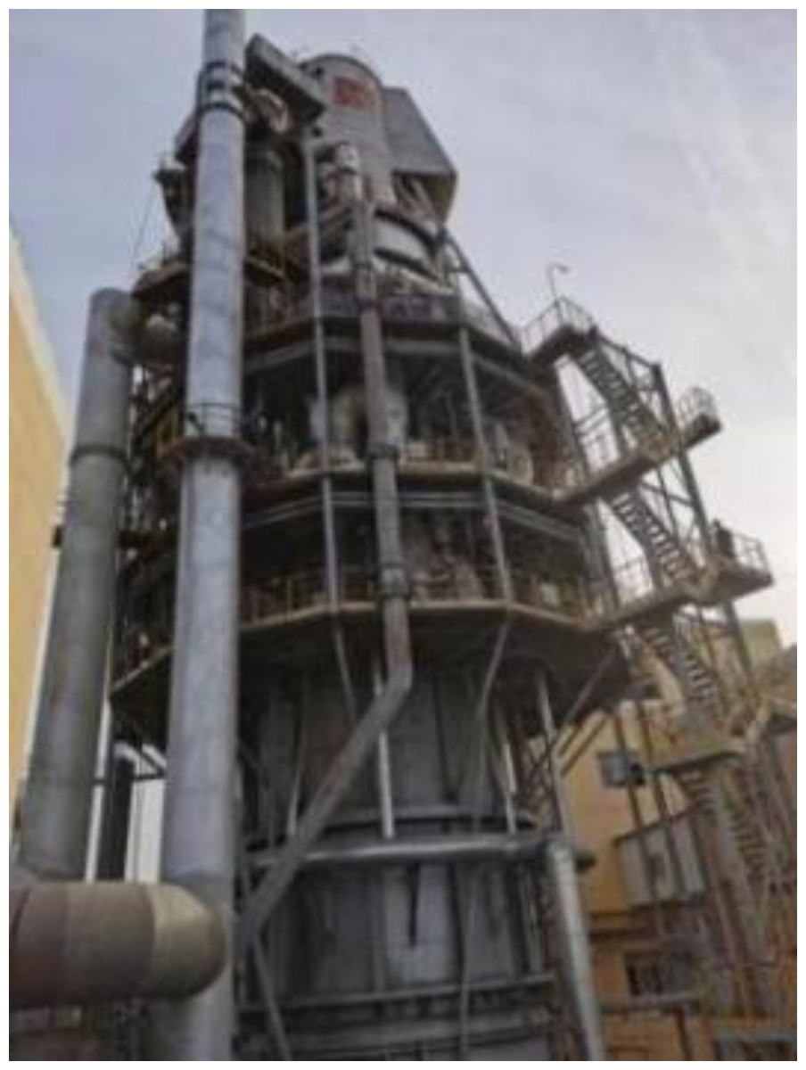
Figure 3: Sleeve kiln with thermal cycle from the Jie Neng Company.
Photograph by Hua Guo.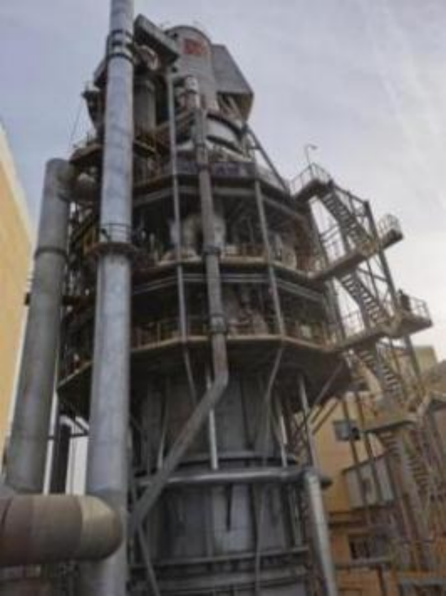
| Variables | Measured variable | Abbreviation |
Numerical example |
Unit |
Gray relative correlation degree |
|---|---|---|---|---|---|
| x1 | Upper arch bridge temperature | TUAB | 231.500 | °C | 0.8609 |
| x2 | Lower arch bridge temperature | TLAB | 173.167 | °C | 0.6885 |
| x3 | Circulating gas temperature | TCG | 747.667 | °C | 0.7838 |
| x4 | Lower combustor temperature | TLCC | 1216.500 | °C | 0.9143 |
| x5 | Outlet temperature of heat exchanger exhaust gas | TEXGHE | 360 | °C | 0.8047 |
| x6 | Inlet temperature of heat exchanger exhaust gas | TENGHE | 615 | °C | 0.7785 |
| x7 | Ring pipe temperature of cooling air | TCAL | 144 | °C | 0.9859 |
| x8 | Mixing temperature of exhaust gas | TEGM | 206 | °C | 0.6957 |
| x9 | Exhaust gas temperature at kiln top | TEGKT | 157 | °C | 0.8715 |
| x10 | Average discharge temperature | TEC | 136 | °C | 0.6986 |
| x11 | Upper combustor gas flow rate | FUCCG | 485 | Nm3/h | 0.8886 |
| x12 | Lower combustor gas flow rate | FLCCG | 756 | Nm3/h | 0.9883 |
| x13 | Upper cold flow rate | FCU | 2,946 | Nm3/h | 0.8414 |
| x14 | Lower cold flow rate | FCL | 10,856 | Nm3/h | 0.5169 |
| x15 | Air flow rate for cooling lime | FLCA | 9,925 | Nm3/h | 0.5302 |
| x16 | gas flow | FG | 9,000 | Nm3/h | 0.6472 |
| x17 | Driving fan flow | FDF | 7,656 | Nm3/h | 0.8597 |
| x18 | Limestone weight per car | ILS | 108 | kg | 0.7538 |
| x0 | Yield | YI | 20.83 | t/2 h |
| Yield classification | Yield characteristics | Parameter characteristics |
|---|---|---|
| YO1 | ≥95% YImax | Normal, optimal operation, no failure |
| YO2 | YImax∈(95%, 85%] | Small gap between the average value and the optimal parameter, no failure |
| YO3 | YImax∈(85%, 75%] | Obvious gap between the average value and the optimal parameter, but no failure occurred |
| YO4 | YImax∈(75%, 65] | Large gap with the average value of the optimal parameter, In the debugging phase |
| YO5 | YImax∈(65%, 0] | Large gap with the average value of the optimal parameter, and a fault occurs |
For measurement accuracy, the measuring elements were evenly distributed at the corresponding positions, including six upper and six lower arch bridge temperatures, six circulating gas and six lower combustor temperatures, and three upper inner cylinder bottom temperatures (these measured variables were averaged before the calculation). In addition, the actual production data also includes the combustion chamber gas flow, exhaust gas temperature in and out of the heat exchanger, average discharge temperature, cooling-air flow rate, exhaust gas mixing temperature, exhaust gas temperature at the kiln top, yield, and limestone weight per cart.
A total of 1,296 amples of measurement variables were analyzed to calculate the gray relative correlation degree with yield using Eq. (1). Variables with high relative correlation were chosen for the initial dataset to reduce computation time and cost. The data were centralized and normalized by scaling the data to [0,1] based on the maximum value of the feature data column to improve the effectiveness of machine learning.
To enhance the generalization ability of the model, dropout and regularization were adopted in this study to prevent overfitting. Dropout randomly disregards some neurons during trainin. This can be combined to form models with stronger predictive power. Most CNN studies that use the ReLU add dropout technology have achieved good classification performance (Paul, Upadhyay & Padhy, 2022).
Yield classification prediction
Selection of data sets
In actual production, owing to the difference in raw material quantity, fuel quantity, reaction temperature, and other parameters, the product output difference is more obvious. Determining whether it is qualified or faulty cannot accurately reflect the actual production situation.
The majority of the data is relatively concentrated, consistent with situations of normal production and good or excellent yields. However, the remaining dispersed portion exhibits several scenarios. Some parameters fall outside the threshold range, others deviate significantly from the average values, and some parameters are close to the lower threshold. When analyzing the actual production data, apart from the situations already detected as faults by the existing control system, the yields could potentially manifest in five scenarios: zero or extremely low, relatively low, not high, good, and excellent. The yield prediction model in this study divides the yield into five categories according to the actual production yield as follows in Table 4.
Utilizing actual production operation data, 1,296 sets of measured parameters were randomly selected as variable samples to validate the effectiveness of the non-optimal operating condition yield prediction method proposed in this chapter.The measured variables with relative correlation degree greater than 75% with yield were selected, including: TUAB, TCG, TLCC, TEXGHE, TENGHE, TCAL, TEGKT, FUCCG, FLCCG, FCU, FDF, ILS. In the following experiments, we used the random split approach to evaluate different methods: a total of 1,296 × 12 samples were randomly selected, where 75% were used for training and the rest for testing.
Comparison for different gray relative correlation degrees
We compared the results of the models using different numbers of measured variables. All measured variables (57 variables), 18 variables (r0 > 50%), 16 variables (r0 > 60%), 12 variables (r0 > 75%), and nine variables (r0 > 80%) were selected for computation, as shown in Table 5. As the number of variables decreased, the computational speed improved significantly. The loss of the datasets with filtered initial variables was significantly lower than that of the datasets containing all variables. The change curves are shown in Fig. 4. As shown in the figure, the model with all measured variables fluctuates more during the calculation process and is stable for a longer time. The margin of accuracy was small. This shows that the variable set screened by the gray correlation calculation has little influence on the accuracy of prediction, whereas the loss and the calculation cost are significantly reduced, and the efficiency is also improved.
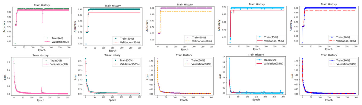
Figure 4: Accuracy and loss for different numbers of measured variables.
(A) 57 variables (All measured variables) (B) 18 variables (ro > 50%) (C) 16 variables (ro > 60%) (D) 12 variables (ro > 75%) (E) nine variables.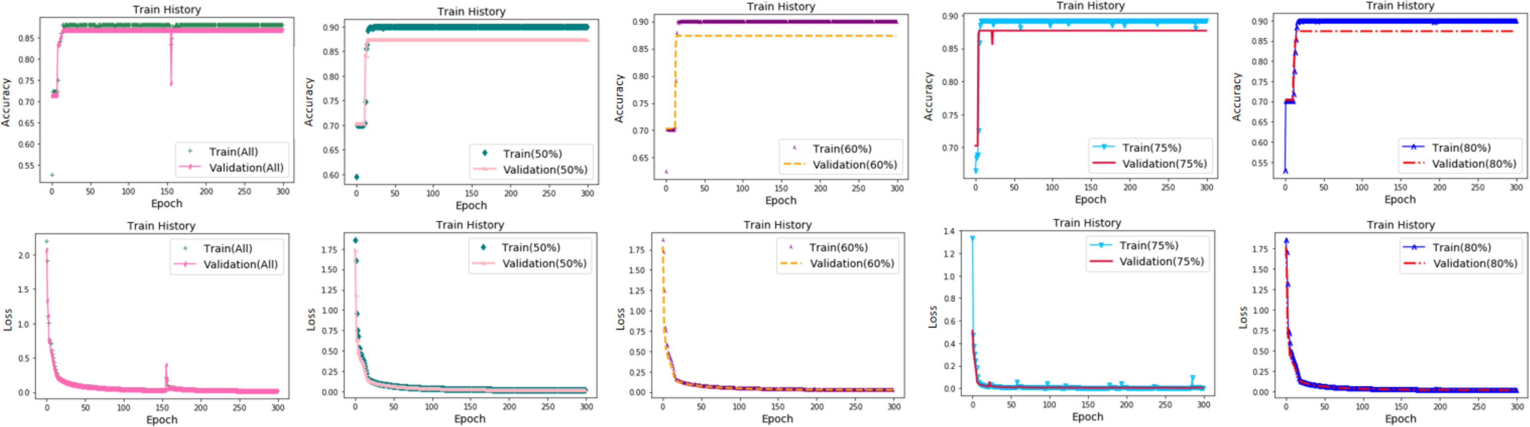
Performance comparison with other methods
To compare the performance of the GCM Net, we conducted extensive experiments in which five methods were used on industrial datasets for multiple classification forecasting. The five methods were MLP, RNN, LSTM, GRU, and CNN.
In this study, each model uses a dataset that has been calculated and screened with a gray relative correlation degree and then preprocessed. All models adopted a sparse_categorical_crossentropy loss function to describe the solution accuracy of the problem. We used the Reduce LR on the Plateau callback function to continuously reduce the learning rate in the training process and obtain the optimal model quicker and accurately.
The output dimensions of the MLP model with three hidden layers were 240, 80, and 20. For both the LSTM and RNN models, there were two hidden layers, and the dimensions of the tensors were 11. The size of the output array in the LSTM was (*, 500) and (*, 250). The size of the output array in the RNN was (*, 880) and (*, 88). For a GRU with one hidden layer, the size of the output array was (*, 256). We performed dropout after each layer for the RNN, LSTM, and GRU. The activation functions of the hidden layers in the adopted ReLU, and the activation function of the output layer used softmax.
As shown in Fig. 5, the performance of the six models in the loss from good to bad showed the following trend: GCM, CNN, GRU, MLP, RNN, and LSTM. The loss curves of GCM, CNN, GRU, and MLP were similar. The lowest value was obtained for GCM (0.0359), followed by CNN (0.0368). However, RNN and LSTM had significantly high losses and poor performance, where the highest loss was observed for LSTM (1.2365), and could not easily fit the trend of local changes in the real values. The loss values for each model are listed in Table 6.
| Number of variables |
Gray relative correlation degreesr0 |
Loss | Accuracy |
Computation speed (µs/sample) |
|---|---|---|---|---|
| 57 | All variables | 0.0630 | 0.8907 | 179 |
| 18 | >50% | 0.0315 | 0.8715 | 85 |
| 16 | >60% | 0.0366 | 0.8715 | 57 |
| 12 | >75% | 0.0359 | 0.8827 | 48 |
| 9 | >80% | 0.0434 | 0.8715 | 46 |
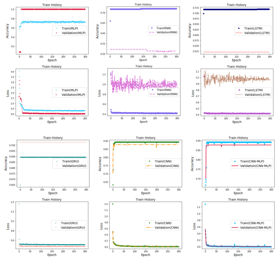
Figure 5: Accuracy and loss of different algorithms.
(A) MLP (B) RNN (C) LSTM (D) GRU (E) CNN (F) CNN-MLP.
The accuracy rates of the six models compared, from high to low, were in the following order: GCM, CNN, MLP, LSTM, RNN, and GRU. The highest rates were observed for GCM and CNN (0.8827) and the lowest for GRU (0.6358). The accuracies of the GCM and CNN were significantly higher than those of the other four models. GCM and CNN performed best when comparing the accuracy of the training and prediction sets. These two models were very similar, and the accuracies of the training and prediction sets were similar. The predicted value coincided well with the actual value, with a smaller deviation. Overfitting was not observed. However, the other four models performed significantly worse.
In terms of model calculation speed, MLP (38 µs/sample) was the fastest among the six models, because it had the simplest and least calculation amount. This was followed by CNN (40 µs/sample) and GCM (48 µs/sample); GCM was slightly slower than CNN, because there were two more hidden layers of MLP. The slowest was RNN (56 µs/sample).
In terms of the stability of the loss calculation, GCM is the best, and the model basically has no fluctuation after 150 calculations. CNN still shows obvious fluctuations after 400 iterations of model calculation, although it performs slightly better than GCM in other aspects. The other four models performed the worst.
It was observed that GCM exhibited the best general performance in predicting the yield classification of calcined lime kilns by thermal cycling.
The experimental results presented above indicate that both the RNN model and the LSTM model are ineffective in extracting crucial features for accurate prediction of lime production yield. Similarly, the MLP and GRU models exhibit only moderate feature extraction capabilities with unsatisfactory detection and prediction effects. Although their stability has improved, their generalization performance remains suboptimal. On the other hand, the CNN and GCM models exhibit superior feature extraction capabilities when applied to lime production data, yielding optimal identification and prediction results along with better generalization performance. In particular, the GCM model outperforms the CNN model in terms of stability. Compared to all of the aforementioned comparative models, the GCM model proposed in this article significantly reduces loss and computational cost while improving prediction efficiency. It has higher accuracy rates, lower losses, superior feature extraction capabilities, better prediction effects, improved generalization performance, as well as improved stability.The GCM hybrid deep learning network yield prediction method effectively, quickly and stably predicts yield classifications, while providing a basis for intelligent yield control.
| Methods | Loss | Accuracy |
Computation speed (µs/sample) |
|---|---|---|---|
| MLP | 0.3229 | 0.7370 | 38 |
| RNN | 1.1933 | 0.6772 | 56 |
| LSTM | 1.2365 | 0.6780 | 50 |
| GRU | 0.3879 | 0.6358 | 52 |
| CNN | 0.0368 | 0.8827 | 40 |
| CNN-MLP | 0.0359 | 0.8827 | 48 |
However, during the model training process, the GCM model requires more extensive debugging of hyperparameters, resulting in increased time consumption. As the dataset size, feature complexity, and number of network layers and units increase, the time required to build a well-performing model also increases. In addition, further improvements in model accuracy may not be achievable.
Non-fault state control strategy and yield increase
Non-fault state control strategy
Lime calcination is a relatively slow production process. Only when there is a fault can the staff adjust the parameters or operating the actuators in a timely manner. In addition, it is difficult to make timely operation to control the yield in the face of a variety of parameters within the threshold range.
Some of the parameters have low relative correlation with the output, or have good stability in the production process. Meanwhile, in order to improve the operability and speed of debugging, production process parameters with relative correlation degree of more than 80% with yield were selected for statistics and comparison. In some cases of failure, there is no yield, according to the original automatic control system to adjust. This article will not be discussed.
There are nine kinds of operation parameters whose relative correlation degree with yield is more than 80%, respectively TUAB, TLCC, TEXGHE, TCAL, TEGKT, FUCCG, FLCCG, FCU and FDF. We have divided the yield operation into YO1,YO2,YO3,YO4 and YO5 according to the yield (see Table 7 for specific production ranges). We compared the corresponding operation parameters according to the yield operating class and characteristics, as shown in Fig. 6.
|
Yield operating class (Yield range) |
Parameter | TUAB | TLCC | TEXGHE | TCAL | TEGKT | FUCCG | FLCCG | FCU | FDF |
|---|---|---|---|---|---|---|---|---|---|---|
| YO1 (Y Imax ∈ [95%, 100%]) | Minimum value | 182.167 | 780.167 | 269.000 | 110.000 | 111.000 | 214.000 | 356.000 | 2014.000 | 3583.000 |
| Maximum value | 278.000 | 1363.167 | 487.000 | 177.000 | 226.000 | 687.000 | 1186.000 | 4020.000 | 8373.000 | |
| Average value | 240.417 | 1204.232 | 374.214 | 137.060 | 160.785 | 482.156 | 711.817 | 3448.131 | 6568.884 | |
| YO2 (Y Imax ∈ (95%, 85%]) | Minimum value | 230.333 | 1010.833 | 343.000 | 111.000 | 120.000 | 417.000 | 522.000 | 2865.000 | 6073.000 |
| Maximum value | 279.667 | 2865.833 | 403.000 | 163.000 | 201.000 | 765.000 | 1073.000 | 3782.000 | 8363.000 | |
| Average value | 249.496 | 1221.687 | 379.710 | 145.355 | 172.629 | 457.258 | 731.113 | 3328.435 | 6912.750 | |
| δ2 | 3.776% | 1.449% | 1.469% | 6.052% | 7.367% | 5.164% | 2.711% | 3.471% | 5.235% | |
| Control priority III | Control sequence | 5 | 9 | 8 | 2 | 1 | 4 | 7 | 6 | 3 |
| YO3 Y Imax ∈ (85%, 75%) |
Minimum value | 238.833 | 642.167 | 349.000 | 120.000 | 93.000 | 1.100 | 152.000 | 2038.000 | 3.000 |
| Maximum value | 247.333 | 1228.667 | 393.000 | 155.000 | 209.000 | 440.000 | 654.000 | 3098.000 | 8408.000 | |
| Average value | 244.198 | 1087.222 | 360.810 | 142.333 | 183.238 | 323.129 | 486.000 | 2910.524 | 6267.190 | |
| δ3 | 2.203% | 11.166% | 5.051% | 2.205% | 6.598% | 27.819% | 34.435% | 12.120% | 9.828% | |
| Control priority III | Control sequence | 9 | 4 | 7 | 8 | 6 | 2 | 1 | 3 | 5 |
| YO4 (Y Imax ∈ (75%, 0)) |
Minimum value | 153.339 | 304.287 | 267.719 | 67.368 | 217.614 | 41.767 | 158.766 | 3006.635 | 208.421 |
| Maximum value | 78.333 | 198.333 | 131.000 | 32.000 | 165.000 | 1.000 | −1.340 | 17.200 | 0.000 | |
| Average value | 249.167 | 817.000 | 395.000 | 220.000 | 388.000 | 110.000 | 199.000 | 3141.000 | 11738.000 | |
| δ4 | 36.220% | 74.732% | 28.458% | 50.848% | 35.345% | 91.338% | 77.696% | 12.804% | 96.827% | |
| Control priority I | Control sequence | 6 | 4 | 8 | 5 | 7 | 2 | 3 | 9 | 1 |
| YO5 (Y I= 0) |
Disparity with the optimal parameter average, fault Operation parameter adjustment by original control system |
|||||||||
Notes:
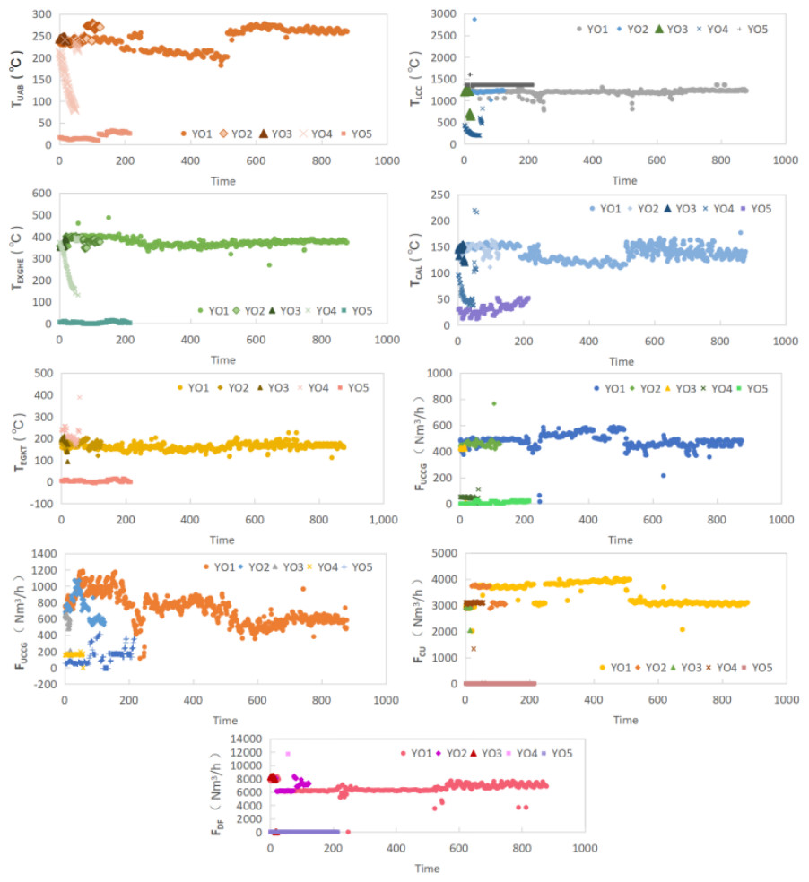
Figure 6: The parameter distribution of different operating conditions corresponding to the yield operating classes.
From Fig. 6, it can be seen that the following classes have obvious differences with the optimal average value in different operating conditions: YO4 in TUAB and TEXGHE, YO3,YO4 in TLCC, FUCCG, FLCCG and FCU, YO2, YO4 in TCAL, TEGKT and FDF.
The maximum, minimum and average values of nine operation parameters for five yield operating classes are listed in Table 7. And the relative error δi between the average value of YO2\3\4 and YO1 in each operating condition.
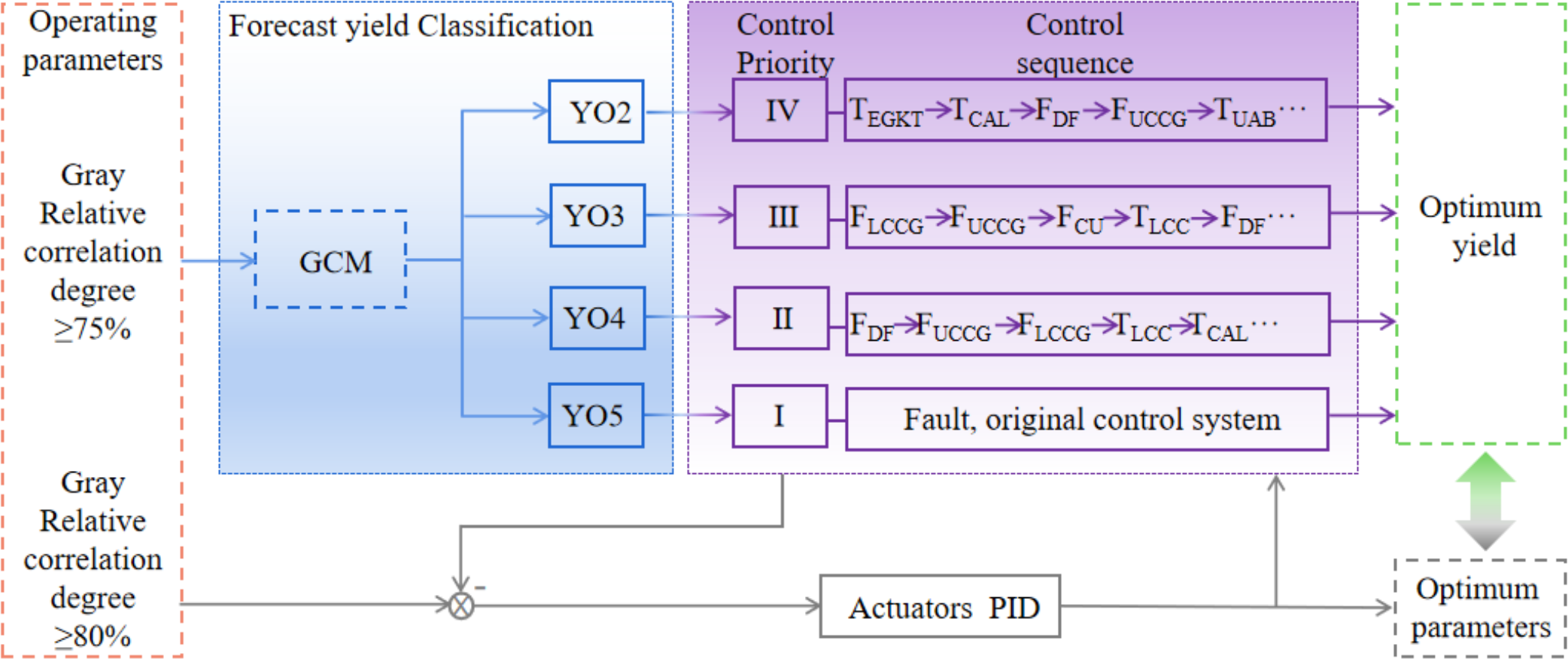
When the yield operating class is YO2, it is close to the optimum yield. There is a small difference between the average values of operation conditions and those of YO1, as shown in Table 7. The control priority is IV and the operating parameters are locally adjusted. The order of regulation is consistent with δ2, as shown in Table 7.
When the yield operating class is YO3, as shown in Table 7, there is a certain gap with the optimal yield, and the average value of some operating parameters is significantly different from that of YO1. At this time, the regulation priority is III, and the regulation order is consistent with δ3.
When the yield operating class is YO4, the gap with the optimum parameters is significant, see Table 7. The control priority is II, and the regulation sequence is sorted according to δ4. Most of the production is in the commissioning stage, and the yield is small. However, through the control sequence of priority II, a debugging guidance can be given to the staff, so as to debug the operation condition faster and reduce the waste.
When the yield operating class is YO5, there is no yield. In this case a fault occurs. The control priority is I. The operating parameters are adjusted according to the original control system.
In the production process, according to a group of data detected by the system sensor, the trained yield prediction model is used to calculate the data and predict the yield classification. The operator or control system can be informed of the yield classification in this set of parameter states in a timely manner. Then perform corresponding operations according to different categories. The parameters of YO1 are taken as the expected value for each controlled quantity and the corresponding actuator is adjusted. Intelligent control strategy is shown in Fig. 7.
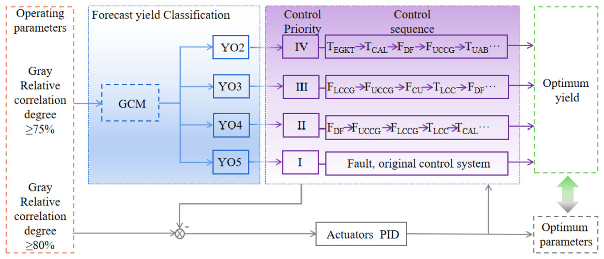
Figure 7: Intelligent control strategy.
Effect on the yield
The average yield of each operating class and the percentage of the total yield are shown in Table 8. In situations requiring adjustment, YO2 accounted for 9.79% and YO3 accounted for 5.04%. In both cases, there was no fault in the production process. It can be adjusted according to the control priority sequence.
When production is calculated based on 100 days,
The yield increase of YOi class Y i is:
Considering that the accuracy of the yield prediction model is 88.27%, it is estimated that the yield can be increased by 1090.699 t/100 days, making minor local adjustments to the operating parameters. The energy conservation is relatively obvious.
The proposed approach combines a yield prediction model with an intelligent decision making method. By utilizing a non-optimal yield classification prediction model trained with actual production data, the variable parameters of the production process can be predicted. This enables timely knowledge of the yield classifications for a given set of parameter states, allowing for intelligent decision-making strategies to be implemented accordingly. Analysis of real production data verifies the feasibility and potential annual yield increase of this intelligent decision-making method. During the production process, system sensors collect a set of data that is then used by a trained yield prediction model to calculate and predict the yield classification. Technicians can promptly identify the yield classification in this specific set of parameter states and subsequently perform appropriate regulation and control operations based on different categories. This ensures that the optimal operational state is achieved as quickly as possible, resulting in increased output while reducing unit energy consumption.
| Yield operating class | YO1 | YO2 | YO3 | YO4 |
|---|---|---|---|---|
| Average yield Ya (t/2h) | 21.183 | 19.233 | 17.932 | 5.843 |
| Percentage of total yield Yt% | 67.80% | 9.79% | 5.04% | 4.40% |
| Yield increase Yi (t/100 days) | 0 | 229.086 | 196.602 | 809.952 |
Conclusion
In this study, we present a GCM model for predicting yield classification. Based on this, intelligent control strategy for the production parameter is proposed. By calculating the actual production data for a lime kiln, it is expected to increase the production by 1090.699 t/100day.
Because there are many variables related to the yield in the production process, which affect the speed and accuracy of the model calculation, we first use the gray relative correlation degree to calculate the correlation degree between variables and yield, and select the variables with a higher correlation degree for model calculation. We compared the calculations and predictions of the models that included different variables. The results show that the loss and calculation time of the model based on the screened variable set were significantly reduced, and the accuracy was almost unaffected. Then, the preprocessed datasets are fed into a hybrid deep network model based on the CNN and MLP networks to predict yield classifications. We conducted extensive experiments using five methods on industrial datasets for multiple classification forecasting to compare the performance of the CNN-MLP model. The results show that CNN-MLP exhibited outstanding performance. Given these results, we can conclude that the GCM model can be applied to yield classification predictions for lime kilns. Then, non-fault state intelligent control priority is set by predicting the yield classification, and the control sequence of operating parameters is given according to different conditions. In the case of no failure or obvious problems, the system or technical staff can decide whether to adjust the unsatisfactory parameters in time according to the prediction results and parameters of each production link in the early stage of production. This allows for higher yields can be achieved to improve production efficiency and reduce unnecessary waste. Simultaneously, it contributes to building intelligently controlled production process systems as an important part of Industry 4.0.
However, there are still some deficiencies in this study and further research is required. Due to the high similarity of operating parameters corresponding to the output category and the crossover phenomenon of parameters between categories, finer categorization has been sacrificed in the pursuit of accurate identification of operating conditions. As a result, the accuracy of control of adjustment amounts during control cannot be improved. In future research efforts, we can improve the performance of the recognition model by considering both the amount of collected running parameters and performing feature analysis on differential parameters. In addition, an attempt should be made to explore various deep learning models to improve the accuracy of recognizing yield classification conditions.
The yield classification prediction method proposed in this article requires the model to be trained using a substantial amount of production operation parameter data prior to regulation. Then, real-time production variables are used to predict production conditions accurately or even in real time. Although our proposed condition detection model does not have a slow computational speed, it still lags behind somewhat; in addition, actual production may introduce parameters that have not previously appeared in our model data set. Ensuring timely or even real-time accurate feedback on yield and quality is an essential aspect for future research efforts. In addition, the use of deep learning predictive models for real-time intelligent online control of capacity and quality is a primary direction for future investigation.