
Autonomous vehicle surveillance through fuzzy C-means segmentation and DeepSORT on aerial images
- Published
- Accepted
- Received
- Academic Editor
- Aswani Kumar Cherukuri
- Subject Areas
- Artificial Intelligence, Autonomous Systems, Computer Vision, Security and Privacy
- Keywords
- Aerial images, Fuzzy C-means, DeepSORT, Smart traffic monitoring, FCM
- Copyright
- © 2025 Qureshi et al.
- Licence
- This is an open access article distributed under the terms of the Creative Commons Attribution License, which permits using, remixing, and building upon the work non-commercially, as long as it is properly attributed. For attribution, the original author(s), title, publication source (PeerJ Computer Science) and either DOI or URL of the article must be cited.
- Cite this article
- 2025. Autonomous vehicle surveillance through fuzzy C-means segmentation and DeepSORT on aerial images. PeerJ Computer Science 11:e2835 https://doi.org/10.7717/peerj-cs.2835
Abstract
The high mobility of uncrewed aerial vehicles (UAVs) has led to their usage in various computer vision applications, notably in intelligent traffic surveillance, where it enhances productivity and simplifies the process. Yet, there are still several challenges that must be resolved to automate these systems. One significant challenge is the accurate extraction of vehicle foregrounds in complex traffic scenarios. As a result, this article proposes a novel vehicle detection and tracking system for autonomous vehicle surveillance, which employs Fuzzy C-mean clustering to segment the aerial images. After segmentation, we employed the YOLOv4 deep learning algorithm, which is efficient in detecting small-sized objects in vehicle detection. Furthermore, an ID assignment and recovery algorithm based on Speed-Up Robust Feature (SURF) is used for multi-vehicle tracking across image frames. Vehicles are determined by counting in each image to estimate the traffic density at different time intervals. Finally, these vehicles were tracked using DeepSORT, which combines the Kalman filter with deep learning to produce accurate results. Furthermore, to understand the traffic flow direction, the path trajectories of each tracked vehicle is projected. Our proposed model demonstrates a noteworthy vehicle detection and tracking rate during experimental validation, attaining precision scores of 0.82 and 0.80 over UAVDT and KIT-AIS datasets for vehicle detection. For vehicle tracking, the precision is 0.87 over the UAVDT dataset and 0.83 for the KIT-AIS dataset.
Introduction
The number of vehicles on the road rises exponentially with rapid economic and population growth. Road traffic monitoring is essential for analyzing traffic data and optimizing roadway operations, making it a key component of intelligent transportation systems (Dikbayir & Bulbul, 2020). It helps identify congestion hotspots, track vehicles, and analyze parking (Weng, Kuo & Tu, 2006; Wu & Yang, 2007; Luo et al., 2021; Puertas et al., 2022).
Recently, uncrewed aerial vehicles (UAVs) have gained popularity for capturing visual data using mounted cameras and computer vision-based object detection (Najiya & Archana, 2018). Aerial imaging applications include road inspection, crowd management, agriculture monitoring, and land use analysis (Schreuder et al., 2003; Ke et al., 2017; Bozcan & Kayacan, 2020; Omar et al., 2021). The portability, affordability, and adaptability of UAVs make them effective for traffic data collection and emergency response (Ringwald et al., 2019; De Moraes & De Freitas, 2020).
Aerial images cover vast areas, including complex backgrounds like trees, highways, and buildings, making object detection challenging. However, advancements in computer vision and deep learning enable efficient detection even in such conditions (Ahmed, Jalal & Rafique, 2019). This article focuses on vehicle detection and tracking for intelligent traffic monitoring using aerial images. Our proposed model segments images to reduce background complexity, detect vehicles, and tracks them across multiple frames.
Segmentation is crucial in traffic monitoring via aerial imagery, as it determines how well vehicles are distinguished from complex backgrounds. We used two techniques: random forest (RF) segmentation and Fuzzy C-means (FCM) clustering, each chosen for its strengths. RF, a supervised method, classifies pixels based on predefined features, excelling in structured environments but requiring training data and high computation. FCM, an unsupervised approach, adapts to background variations, enhancing generalizability. Compared to methods like Otsu’s thresholding, K-means, or graph-based segmentation, RF and FCM offer greater adaptability and accuracy in varying lighting and occlusions. Unlike fixed-threshold methods, FCM allows smooth transitions between object and background, while RF ensures context-aware foreground extraction, outperforming purely statistical techniques like K-means.
The RGB images from video sequences are first extracted and preprocessed. Then, segmentation is performed using the FCM technique (Hashemi, Gholian-Jouybari & Hajiaghaei-Keshteli, 2023). The segmented images are fed into the vehicle detection module, where YOLOv4 (Yusuf, Hanzla & Jalal, 2024) detects small objects. To track multiple vehicles across frames, each detected vehicle is assigned an ID using Speed-Up Robust Feature (SURF) (Du, Su & Cai, 2009). A vehicle count is maintained across frames to estimate traffic density. Tracking is achieved via the DeepSORT Kalman filter (Kejriwal et al., 2022). The proposed traffic monitoring system is validated using UAVDT (Yu et al., 2020) and KIT-AIS (Beheim, 2021) datasets, demonstrating superior detection and tracking precision compared to state-of-the-art (SOTA) methods. The key contributions of this work include:
A hybrid model for the detection and tracking of vehicles on roadways for effective monitoring of transportation networks in aerial images having different complexity levels is presented.
A comparison of the random forest (Aroef, Rivan & Rustam, 2020) classifier and unsupervised segmentation technique, i.e., the Fuzzy C-mean algorithm, has been used for segmentation purposes.
We have greatly improved the precision, recall, F1 score, and quality performance measures for vehicle detection and tracking when compared to previous methods.
Vehicle tracking using the DeepSORT algorithm, ID assignment and recovery module based on SURF has been implemented.
The proposed system’s accuracy is validated on three public datasets. The article is structured as follows: “Introduction” introduces the study, “Related Work” covers related work, and “Materials and Methods” details the datasets, methodology, and system architecture. “Datasets Description” presents experiments and results, followed by a discussion in “Results”. “Conclusion and Future Work” concludes with future directions.
Related work
Many researchers have used machine learning for intelligent traffic monitoring, while others focused on deep learning with aerial images. For detection, various hand-crafted features were extracted, including SIFT (Battiato et al., 2007), Histogram of Oriented Gradient (HOG) (Kong et al., 2019; López-Sastre et al., 2019; Jalal, Khalid & Kim, 2020; Rizwan et al., 2023), and Haar-like features (Tang et al., 2017; Shahzad & Jalal, 2021). These feature vectors trained different classifiers but suffered from the curse of dimensionality, making them computationally expensive. Recently, deep learning models have excelled in object detection, especially in complex scenarios. To summarize current techniques, related work is categorized into machine learning- and deep learning-based traffic analysis.
Machine learning-based traffic scene analysis
Machine learning has long been used in computer vision, particularly for traffic monitoring. Rafique et al. (2023) developed a vehicle detection model using Haar-like features and an AdaBoost classifier. Tang et al. (2017) performed detection and classification via background subtraction and SIFT extraction, training neural networks and support vector machines (SVMs). Jabri et al. (2018) used Haar features and local binary patterns (LBP) with an AdaBoost classifier, which, when combined, improved results but increased energy consumption (Akhter, Jalal & Kim, 2021). Charouh, Ghogho & Guennoun (2019) proposed a moving vehicle detection method using background subtraction and morphological corrections. Yu et al. (2003) classified and tracked vehicles via image differencing and a Kalman filter. Mu, Hui & Zhao (2016) identified moving vehicles by selecting high sum of absolute differences (SAD) regions and applying SIFT for matching. Chen, Ellis & Velastin (2012) introduced an urban vehicle detection method using SVM and HOG features. However, these approaches are computationally intensive and struggle with complex scenes, affecting model generalizability.
Deep learning-based traffic scene analysis
Traditionally, traffic monitoring relies on manual methods and in-vehicle technologies. However, deep learning-based image processing has outperformed conventional approaches. Lin & Jhang (2022) proposed a car detection method using the YOLOv4 algorithm. Similarly, Al-qaness et al. (2021) developed a model that processes traffic video sequences with a CNN before applying YOLO for detection, though missing vehicles remain a challenge. Muchtar, Afdhal & Nasaruddin (2020) introduced a YOLOv3-based vehicle detection and classification approach, segmenting images with MOG2 before detection. Ammour et al. (2017) presented a vehicle detection and counting method combining a linear SVM classifier with a pre-trained CNN on high-resolution UAV imagery, but its high computational time limits real-time application.
This research aims to enhance modern computer vision technologies. Our system efficiently detects, tracks, and monitors traffic for intelligent, environmentally aware surveillance. By integrating multiple deep learning methodologies, it surpasses existing car detection and autonomous traffic surveillance systems in performance and accuracy.
Innovation over existing approaches
Our model advances vehicle detection and tracking in accuracy, scalability, and applicability. Unlike handcrafted feature-based methods like HOG-SVM and SIFT, which struggle with occlusions and complex backgrounds, we use YOLOv4, optimized for small object detection. Integrating FCM segmentation before detection reduces background interference, improving precision, recall, and F1-score in aerial imagery.
Many existing methods rely on computationally expensive region-based detectors like Faster region-based convolutional neural network (R-CNN), unsuitable for real-time UAV traffic monitoring. Our pipeline, using YOLOv4 and DeepSORT, is optimized for large-scale, real-time processing, ensuring efficient tracking in dynamic conditions. Unlike ground-based CCTV models, our UAV-specific approach integrates DeepSORT with ID assignment and SURF-based recovery for robust multi-frame tracking. Additionally, our vehicle trajectory estimation module enables a comprehensive analysis of traffic flow patterns, often missing in conventional detection models.
Materials and Methods
This article proposes a multi-stage vehicle recognition and tracking system for aerial images using semantic segmentation. After extracting and preprocessing frames, vehicles are segmented from the background using random forest (RF) and FCM clustering, improving detection by YOLOv4. RF, a supervised method, relies on labeled data, while FCM adapts to background variations without prior training. YOLOv4’s CSPDarknet53 backbone and PANet neck enhance feature extraction for reliable small-vehicle detection. Tracking is achieved using SURF extraction, a burst particle filter for position prediction, and DeepSORT with Kalman filtering for identity consistency in dense traffic. Finally, trajectory estimation maps vehicle movements for traffic analysis. Figure 1 illustrates the proposed system, with subsequent sections detailing each module.
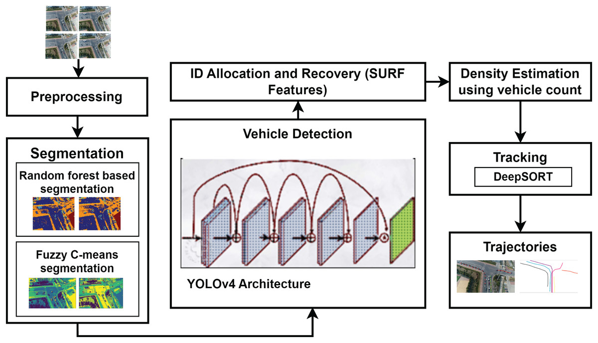
Figure 1: The architecture of the proposed autonomous vehicle surveillance algorithm.
Preprocessing
In the preprocessing step, we extract a series of images from the video to achieve better outcomes for vehicle detection and tracking. Afterwards, each extracted frame is resized to 768 × 768 dimensions. To denoise the image, a nonlinear adaptation known as gamma correction (Xu et al., 2009) is applied to every pixel value using
(1) where I is the input image, G represents the gamma value, which can be obtained using Eq. (2) and O denotes the output image scaled back to [0, 255].
(2) where is the mean of the image after converting it to grayscale. Preprocessing plays a crucial role in enhancing image quality before segmentation, detection, and tracking. In our method, we remove Gaussian noise and motion blur common in UAV-captured imagery using median filtering to preserve edges while eliminating noise artifacts. Additionally, gamma correction is applied to adjust brightness variations caused by aerial lighting conditions. The gamma value (G) is selected adaptively using the formula G = mean ( )/128, where is the grayscale-converted image. This ensures that contrast enhancement is proportional to the image’s overall brightness, preventing overexposure or underexposure.
Semantic segmentation
Segmentation is a crucial preprocessing step in aerial image analysis, isolating vehicles from complex backgrounds to improve object detection efficiency. Aerial images often include irrelevant elements like buildings, vegetation, and shadows, leading to false detections and higher computational costs (Rafique et al., 2022). Using RF and FCM clustering reduces background noise, allowing the model to focus on vehicles. This enhances detection accuracy, minimizes misclassifications, and improves tracking by ensuring consistent vehicle identification across frames.
Random forest-based semantic segmentation
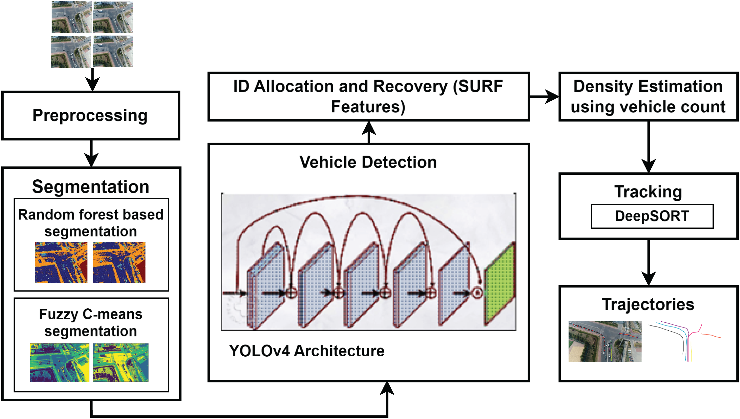
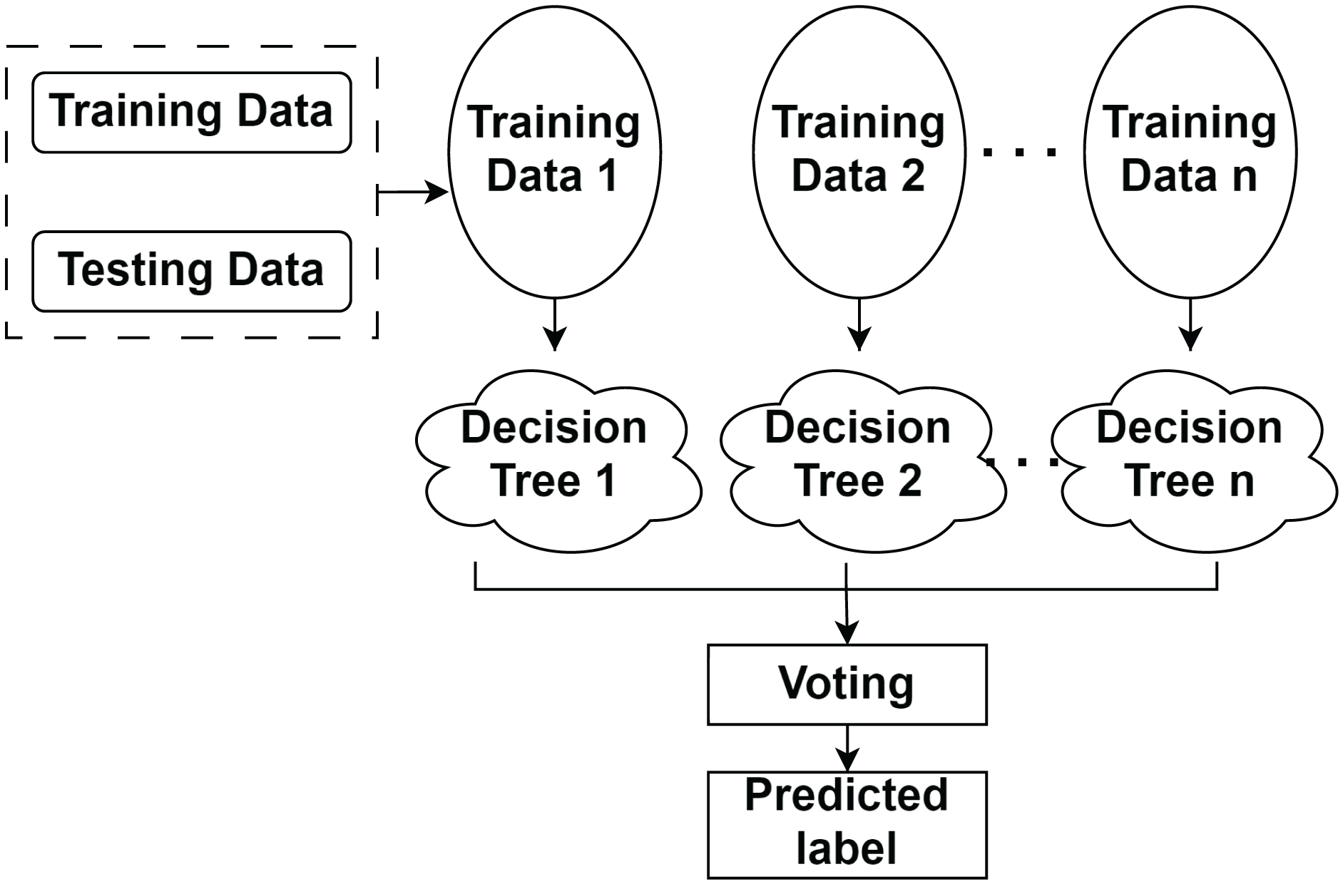
A random forest is a supervised classifier. The first step in segmentation involves extracting a feature vector from images and labels for model training. Feature extraction uses filters such as Canny edge detection (Yuan & Xu, 2016), Prewitt (Chaple, Daruwala & Gofane, 2015), Scharr (Kumar, Lal & Kumar, 2021), and a median filter. RF combines multiple decision trees; each tree outputs a class label, and the label with the most votes becomes the predicted output, as shown in Fig. 2.
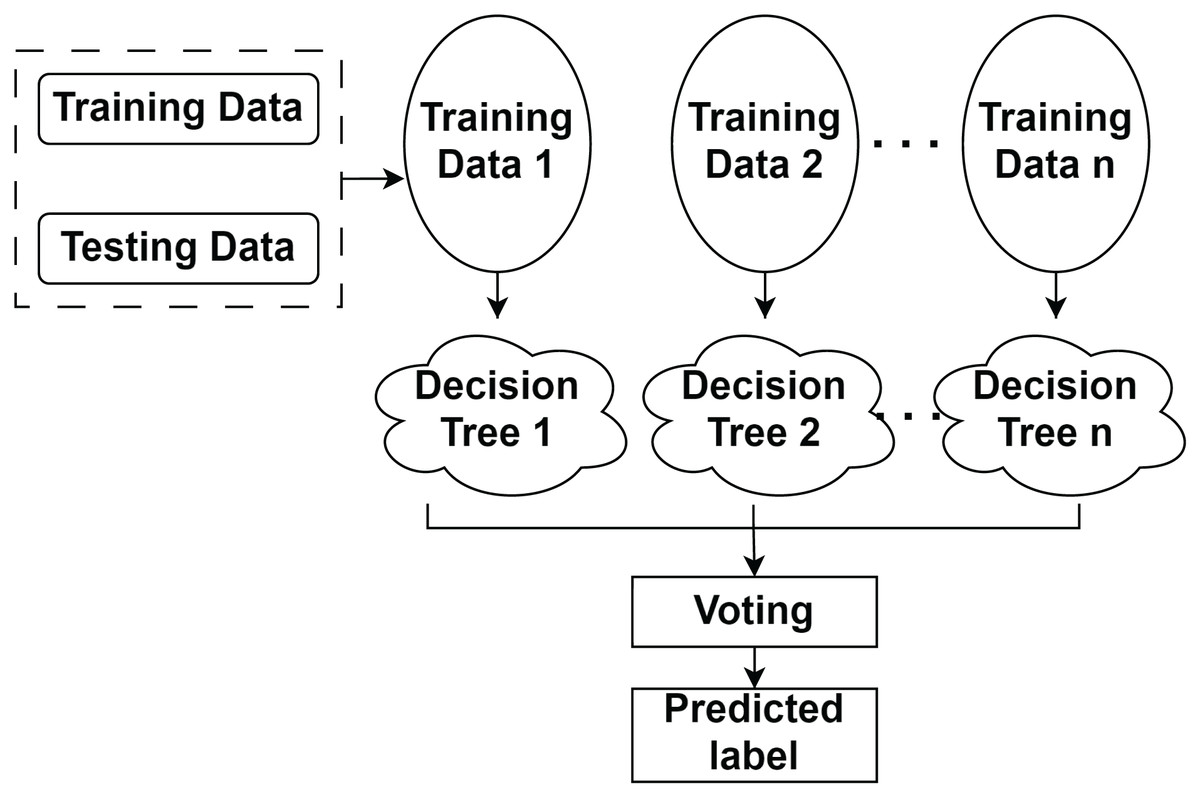
Figure 2: Working methodology of random forest classifier for segmentation.
Each feature’s importance on the decision tree is calculated by Eq. (3).
(3) where represents the importance score of features , denotes the importance contribution of node j that splits on feature I and is the total importance contribution across all nodes k in the tree. Each calculated feature is normalized by using Eq. (4).
(4)
Also, the overall importance of each input feature has been calculated by averaging it over all the Random Forest trees as given in Eq. (5).
(5) where is the overall importance score of feature i in the random forest, represents the normalized importance of feature i in tree j, and T is the total number of trees in the forest.
We trained the model using the leave one subject out (LOSO) validation technique (Pauli, Pohl & Golz, 2021). Figure 3 visualizes the segmentation results: Fig. 3A displays the original frames, while Fig. 3B shows the segmentation using RF.

Figure 3: Segmentation result using random forest classifier.
(A) Original image frames (B) segmentation results.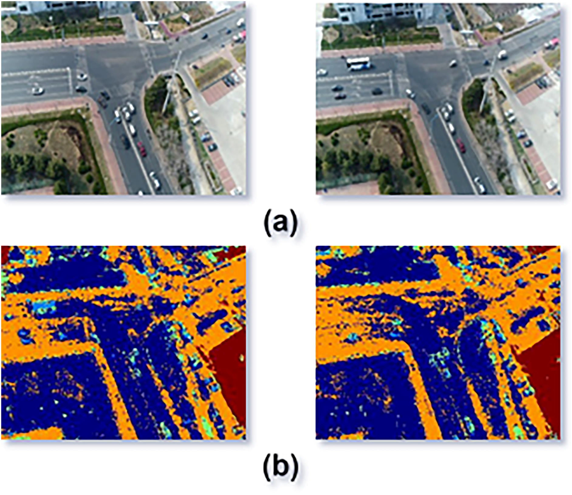
Segmentation using fuzzy C-means algorithm
FCM is a segmentation algorithm where pixels are linked to multiple clusters (Miao, Zhou & Huang, 2020), reflecting fuzzy logic based on co-occurring elements. The objective function is optimized over iterations to complete the segmentation process (Ahmed, Jalal & Kim, 2020). During this process, clustering centers and membership degrees are updated. The performance index K_FCM calculates the weighted sum of distances between elements and cluster centers, as shown in Eq. (6).
(6) where represents the objective function of the FCM clustering algorithm, is the membership degree of data point kkk belonging to cluster i, is the data point, is the center of cluster i, and p is the fuzziness parameter (with 1 < p < ). The degree of membership function satisfies the conditions given in Eq. (7).
(7)
is the feasible membership matrix in the Fuzzy C-Means algorithm, where denotes the membership degree of data point k to cluster i, c is the number of clusters, and N is the total number of data points. The conditions ensure membership values are between 0 and 1, the sum of memberships for each data point across all clusters equals 1, and each cluster has non-zero total membership.
Equations (8) and (9) are used to update the membership matrix and the cluster centres.
(8) where represents the membership degree of data point k to cluster i raised to the power of p, is the distance between data point k and cluster center i, and is the distance between data point k and other cluster centers j. The equation calculates the fuzzy membership based on the relative distances, where p is the fuzziness parameter.
(9) where represents the center of cluster j, is the membership degree of data point k to cluster i raised to the power of p, and is the data point. The equation calculates the weighted average of the data points, with the membership degrees serving as the weights, to determine the new center of cluster j.
Pixels are given high membership values when they are near the centroid of their respective class, and low membership values when they are far from the centroid, thus, the FCM objective function was minimized. The output of the FCM segmentation is shown in Fig. 4. Figure 4A presents the original images whereas the segmented images are shown in Fig. 4B.
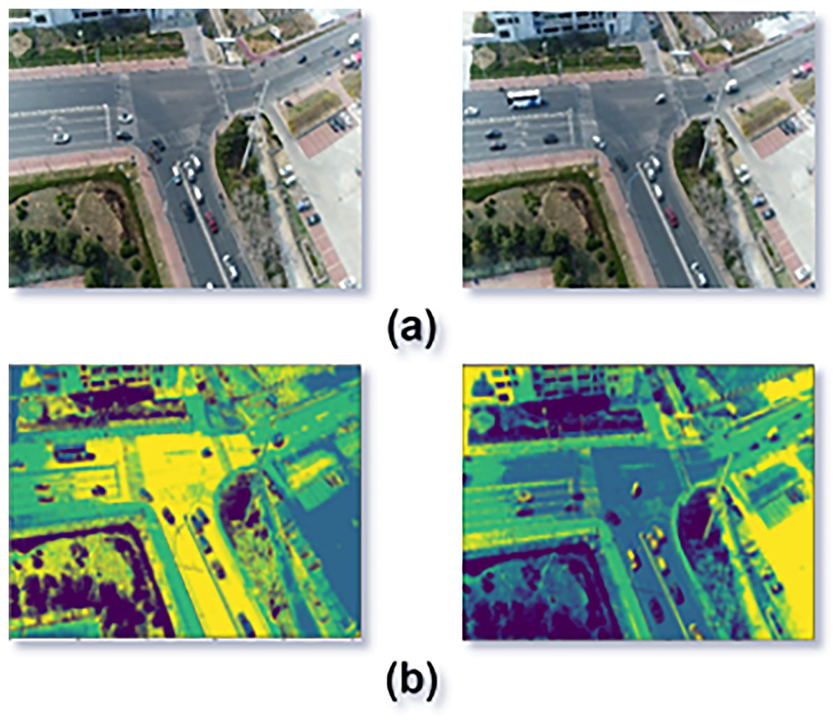
Figure 4: Segmentation result using FCM algorithm.
(A) Original image frames (B) segmentation results.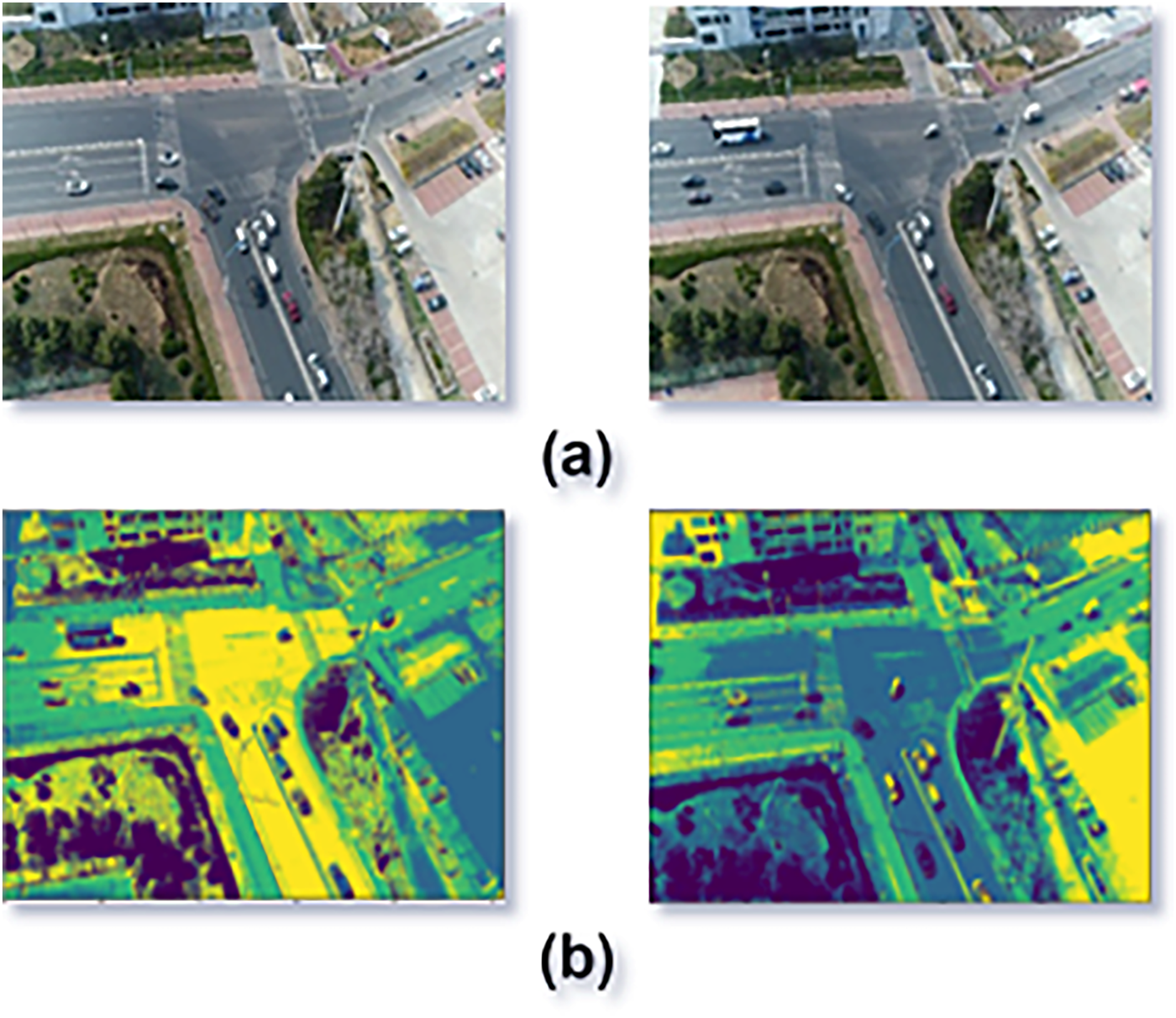
For segmentation, we use RF and FCM to separate vehicles from the background. RF segmentation employs supervised learning with features extracted via Canny edge detection, Prewitt, Scharr, and median filters, classified by an ensemble of decision trees trained using LOSO validation. FCM clustering assigns membership values to pixels, enabling soft clustering that minimizes errors, especially in occluded areas. The computational cost and error rates of RF and FCM are compared using Eq. (10).
(10)
The RF classifier requires training on the ground truth, increasing the model’s computational complexity. In contrast, FCM can be applied without explicit training, enhancing the algorithm’s generalizability. Table 1 shows the error rates for image segmentation using RF and FCM on the UAVDT and KIS-AIS datasets. Considering both computational time and error rates, FCM proves to be more effective and accurate. Therefore, FCMP results are used for further processing, such as vehicle detection, ID allocation, recovery, counting, and tracking. Table 2 shows comparsion of segmentation techniques.
| Datasets | Error rate | |
|---|---|---|
| Random forest | FCM | |
| UAVDT | 0.37 | 0.19 |
| KIT-AIS | 0.43 | 0.24 |
| Datasets | Segmentation accuracies | |
|---|---|---|
| Random forest | FCM | |
| UAVDT | 0.63 | 0.81 |
| KIT-AIS | 0.57 | 0.76 |
Comparison of FCM and RF segmentation
To evaluate the effectiveness of FCM and RF segmentation, we compared their computational efficiency, training dependency, adaptability to varying backgrounds, and robustness against noise. The following Table 3 presents a quantitative comparison based on segmentation performance on the UAVDT and KIT-AIS datasets.
| Datasets | Precision | Recall | F1 score | Quality |
|---|---|---|---|---|
| UAVDT | 0.82 | 0.80 | 0.81 | 0.68 |
| KIT-AIS | 0.80 | 0.81 | 0.80 | 0.67 |
RF segmentation uses hard classification, leading to over-segmentation or misclassification, especially in aerial imagery with shadows and varying lighting. FCM’s soft clustering ensures smoother boundaries, crucial for UAV-based traffic monitoring where motion blur and occlusions affect vehicle edges. Unlike RF, FCM adapts to varying road conditions and shadows, offering greater robustness and reducing segmentation artifacts, thus improving vehicle detection accuracy.
Vehicle detection
After image segmentation, vehicle detection is performed using the YOLOv4 deep learning algorithm, which detects objects with high accuracy and speed. YOLOv4’s architecture includes CSPDarknet53, PANet, and the YOLOv3 head, with CNNs splitting images into regions to predict probabilities. This reduces overfitting by using convolution and fewer parameters, as shown in Fig. 5.
(11)
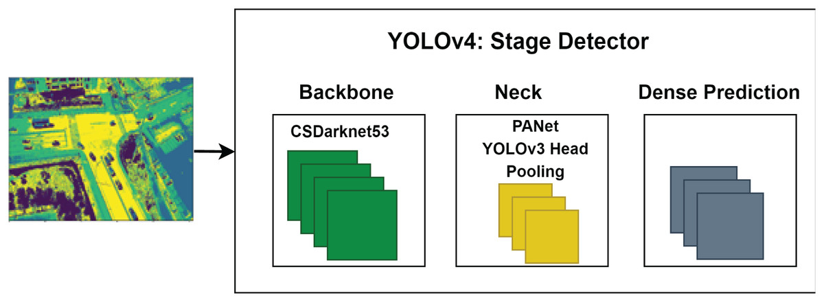
Figure 5: The architecture of YOLOv4 for vehicle detection.
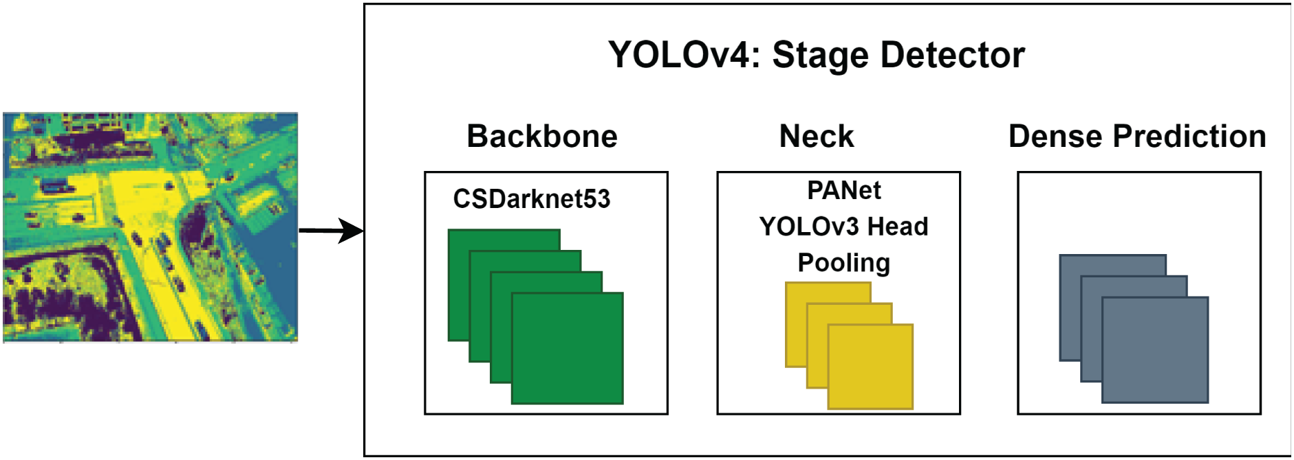
G[i, j] represents the output at position (i, j), h[u, v] is the filter value at (u, v), and F[i + u, j + v] is the input at the shifted position. The equation performs a convolution by summing the product of the filter and input values over a kernel-defined neighborhood. The CNN uses a pooling layer for downsampling, as defined in Eq. (12).
(12) where is the maximum value of the pixel after each iteration. Convolutional and pooling layers work together to facilitate effective feature learning and selection. In the end, the Mish activation function is implemented to get the output label as given in Eq. (13).
(13) where represents the soft plus activation function.
When the performance was compared, YOLOv4 was two times faster than EfficientDet (a competitive recognition model). For vehicle detection, we utilize YOLOv4, which consists of a CSPDarknet53 backbone, a PANet path-aggregation neck, and a YOLOv3 head. We configure YOLOv4 with batch size = 16, momentum = 0.937, learning rate = 0.001, and IoU threshold = 0.5 to balance accuracy and computational efficiency in UAV imagery. Table 4 shows comparsion of YOLOv4 with other methods.
| Datasets | Precision | Recall | F1 score | Quality |
|---|---|---|---|---|
| UAVDT | 0.87 | 0.85 | 0.86 | 0.76 |
| KIT-AIS | 0.83 | 0.80 | 0.81 | 0.69 |
ID allocation and recovery
Each detected vehicle is assigned a unique ID based on SURF features, which provide reliable, scale-invariant, and efficient image comparison (Bay et al., 2008). SURF features are fast to compute, making them suitable for real-time object recognition. The method includes an interest point detector and descriptor (Du, Su & Cai, 2009), with interest points identified using an integral computed by Eq. (14).
(14) where is the integral image at the location and is the input image. Moreover, the blob-like structure in the image is calculated by using the Hessian matrix as given in Eq. (15).
(15) where represents the Hessian matrix at point x with scale σ, is the second derivative of the image with respect to x, is the mixed second derivative with respect to x and y, and is the second derivative with respect to y. The Hessian matrix captures the curvature of the image, which is used in various image processing tasks like edge detection and feature extraction. The assigned IDs can be recovered based on the feature-matching score in the succeeding frame detections.
For ID assignment and recovery, we employ SURF to extract key descriptors for each detected vehicle. An ID is successfully recovered if the number of feature matches between frames exceeds a predefined threshold (set to eight in our experiments). If fewer than eight matches are found, the vehicle is registered as a new entry, ensuring a balance between continuity and robustness in tracking.
Vehicle counting
For traffic situation analysis, vehicle counting is performed in each image frame based on vehicle detections. All the detections made by YOLOv4 are recorded using a counter, as given in Eq. (16). Vehicle counting in each frame estimates traffic density on the road at different time intervals, which can be further used to predict spontaneous reactions to traffic jams or other unhappy incidents.
(16) where T is the vehicle detections in a frame.
Vehicle tracking
To track the movement of vehicles frame by frame, we implemented DeepSORT (Wojke, Bewley & Paulus, 2017; Hou, Wang & Chau, 2019; Kapania et al., 2020; Pramanik et al., 2022). DeepSORT is a tracking algorithm that combines the Kalman filter with deep learning to track objects not only based on their motion and velocity but also on their appearance. The motion information is incorporated using the Mahalanobis distance between the Kalman state and the newly arrived measurement by using Eq. (17).
(17) where represents the Mahalanobis distance between data point and the mean of cluster i, is the inverse of the covariance matrix of cluster i, and is the difference between data point and the cluster center . The equation computes the squared distance, weighted by the inverse covariance, which measures how far is from the cluster center in terms of the cluster’s spread.
The appearance information can be calculated using the minimum cosine distance between i-th and j-th detection in appearance space as
(18) where represents the minimum distance between data point j and the points in cluster i, is the feature vector of data point j, and is the feature vector of a point in cluster i. The equation calculates the minimum value of the distance measure , where is the dot product, and is the set of all points in cluster i, ensuring the closest match in the feature space.
(19) where represents the combined distance measure between data point j and cluster i, is the Mahalanobis distance (as defined earlier), and is the minimum distance measure (as defined earlier). The parameter λ is a weight that balances the contribution of both distance measures, with λ controlling the influence of and (1−λ) controlling the influence of .
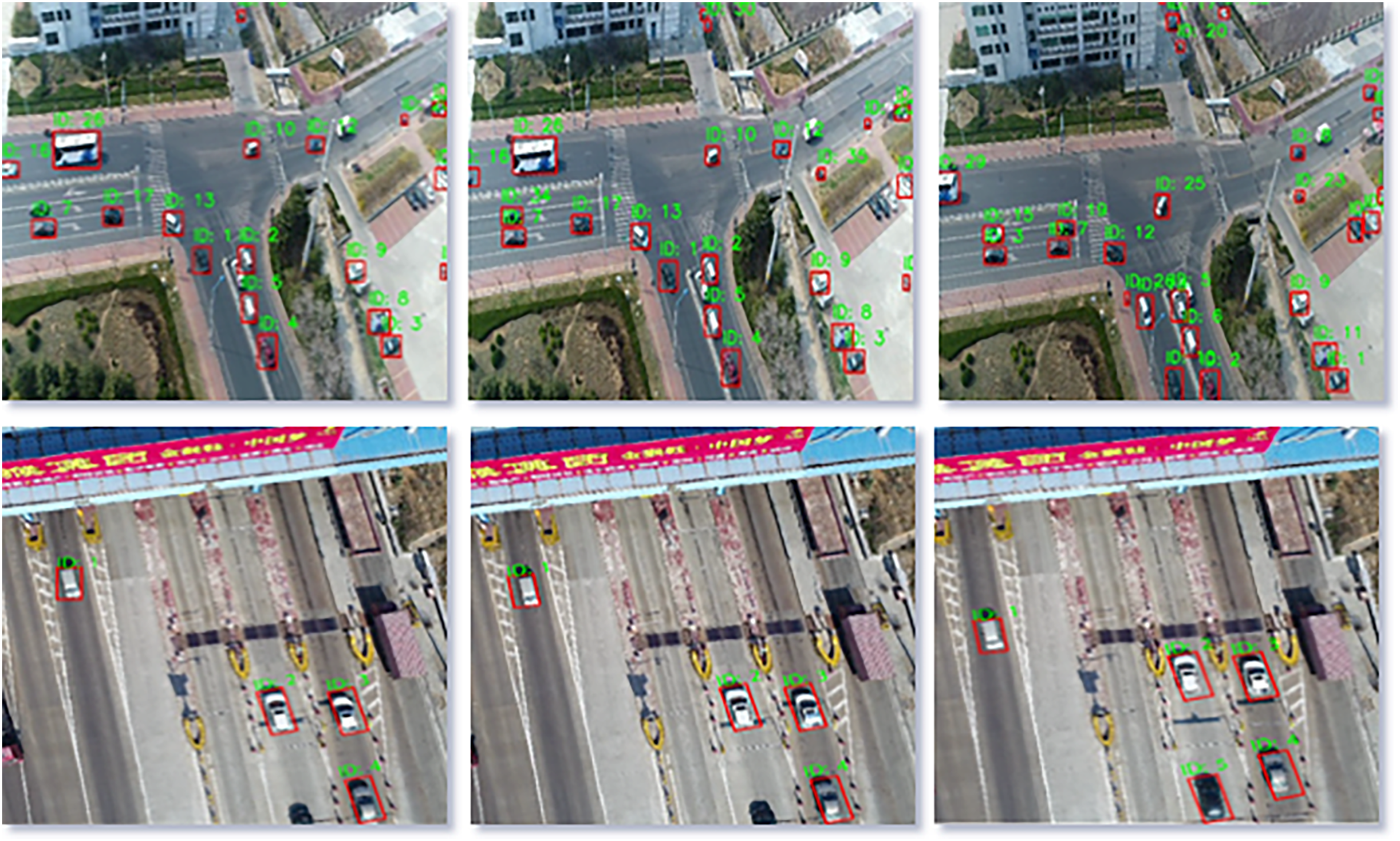
We use a pre-trained CNN model with two convolution layers, one max pooling layer, six residual layers connected to a dense layer, and L2 normalization to calculate the appearance features. Figure 6 shows the tracking results in each succeeding frame.
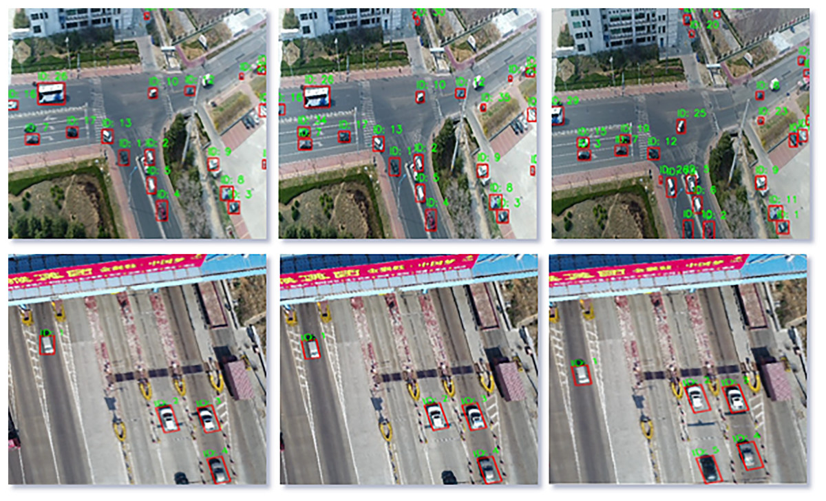
Figure 6: Tracking of multiple vehicles across the image frames extracted from the video.
We integrate DeepSORT, an extension of SORT, by adding deep appearance-based feature extraction with Kalman filtering. The Mahalanobis distance associates new detections with tracklets, while a cosine similarity-based re-identification model maintains tracking consistency when objects temporarily exit the frame. Table 5 shows comparsion of DeepSORT with other techniques.
| Datasets | AID rate (%) | Recovery rate (%) |
|---|---|---|
| UAVDT | 65 | 62 |
| KIT-AIS | 63 | 59 |
Vehicle trajectories estimation
We track vehicle movement by estimating and plotting each vehicle’s trajectory using the geometric coordinates of detected boxes. The DeepSORT algorithm provides the location data, from which we calculate and mark center points. The algorithm inputs detection coordinates into the DeepSORT tracker, which predicts vehicle locations in subsequent frames. SURF features are extracted and matched to recover vehicle IDs. If matches exceed a threshold, the ID is retrieved; otherwise, a new ID is assigned. Rectangular coordinates and midpoints are used to mark vehicle trajectories. Detailed steps are provided in Algorithm 1.
| Input: V // list of rectangular coordinates of length |
| Output: // vehicle trajectories |
| DeepSORT(V) //Estimated positions of vehicles by tracker |
| feature_vector=[] |
| For i = 1 to the length of T |
| new_feature SURF(Ti) |
| If feature_vector==[ ] |
| feature_vector new_feature |
| Else |
| matches (new_feature, feature_vector) |
| If matches > 8 |
| AssignID(Ti) |
| Else |
| feature_vector new_feature |
| ExtractRectangularCoordinatesofVehicle () |
| End for |
| return vehicle trajectories |
Datasets description
For vehicle surveillance, two datasets were used: UAVDT and KIT-AIS datasets. A detailed description of each dataset is mentioned in the following subsections.
UAVDT dataset
The UAVDT dataset (Yu et al., 2020) consists of more than 10 h of video captured using a UAV platform in various urban settings. These traffic scenes include intersections, toll plazas, motorways, crossings, and arterial roadways. The .jpg images have a resolution of 1,080 × 540 pixels, while the videos were shot at a frame rate of 30 (fps).
KIT-AIS dataset
The Karlsruher Institut fur Technologie ¨ Aerial Image Sequences (KIT-AIS) dataset (Beheim, 2021) consists of 299 image frames with .jpg format extracted from video sequences. This dataset is provided by German Aerospace. It consists of five different classes, i.e., cars, truck, bus, minibus, and cyclist.
Dataset partitioning and augmentation strategies
Our study uses two publicly available aerial image datasets: UAVDT and KIT-AIS, each containing varied traffic scenarios. Both datasets were split into training, validation, and test sets as follows:
UAVDT dataset: With its large number of images, we applied an 80-10-10 split (80% for training, 10% for validation, and 10% for testing), ensuring broad training conditions and unbiased performance evaluation.
KIT-AIS dataset: Due to its smaller size, we enhanced the dataset with random rotation (±15°), horizontal flipping, brightness adjustment, and Gaussian noise addition. This augmented the dataset, creating a 70% training, 15% validation, and 15% test split.
We augmented the KIT-AIS dataset with random rotation (±15°), horizontal flipping, brightness adjustment, and Gaussian noise to simulate real-world variations like lighting, vehicle orientations, and image noise. This improved model generalizability, ensuring robust training and evaluation across diverse aerial traffic scenarios.
Results
Experiments were conducted on a Windows 10 (64-bit) system with an Intel Core i5-7200U processor, 8 GB RAM, and an NVIDIA GeForce GTX 1650 GPU (4 GB VRAM) for deep learning acceleration. The model was implemented in Python 3.7 using TensorFlow 2.4.1 (YOLOv4), OpenCV 4.5.1 (image preprocessing), Scikit-learn 0.24.2 (Random Forest segmentation), SciPy 1.6.2 (FCM clustering), and a custom DeepSORT implementation for multi-object tracking.
We employed seven evaluation parameters to assess the performance of our presented methodology. To compare the performance of random forest-based segmentation and FCM segmentation we used the accuracy as given in Eq. (20).
(20) where (TP + FP + FN) is the total area of ground truth and prediction, and TP and TN indicate the area of intersection. However, the effectiveness of vehicle detection and tracking is assessed using four evaluation metrics, namely precision, recall, quality, and F1 score as calculated by using Eqs. (21), (22), (23) and (24).
(21)
Precision measures the proportion of correctly identified vehicles among all detected instances. A high precision score indicates that the system effectively minimizes false positives, ensuring that non-vehicle objects are not mistakenly classified as vehicles.
(22)
Recall represents the proportion of correctly identified vehicles relative to the total number of actual vehicles present in the dataset. A higher recall value indicates that the system successfully captures a greater percentage of vehicles, minimizing false negatives.
(23)
Quality is a holistic performance measure that incorporates the correctness of detections and tracking stability. This metric is particularly relevant to our system as it evaluates how well the detected vehicles are maintained across frames, ensuring consistency in tracking results.
(24)
F1-score is the harmonic mean of precision and recall, providing a balanced measure of the system’s accuracy. Since precision and recall often exhibit a trade-off, F1-score ensures that both aspects are considered, making it a robust evaluation metric for vehicle detection and tracking.
Where is a true positive, denotes true negative, is a false positive, and is a false negative, respectively.
We utilized two new measures to evaluate the ID assignment and recovery module as given in Eqs. (25) and (26). AID is the accurate ID rate, which denotes the percentage of accurate ID numbers allotted to vehicles.
(25) where N is the total number of vehicles. denotes the overall number of ID assignments made to the true vehicles, and denotes all of them. The represents the percentage of true IDs recovered.
(26) where N represents the total number of dissimilar vehicles. represents the i-th number of true recoveries and is the all-existing recoveries.
We compared the random forest and FCM segmentation methods based on accuracy and computational time. While random forest requires custom training, increasing its computational cost, FCM yields better segmentation results. Therefore, FCM was selected for our algorithm. Accuracy results for both methods are shown in Table 6.
| Datasets | Models | Precision |
|---|---|---|
| UAVDT | NDFT (Cao et al., 2020) | 0.520 |
| SpotNet (Perreault et al., 2020) | 0.528 | |
| Our method | 0.82 | |
| KIT-AIS | Beheim (2021) | 0.79 |
| Our method | 0.80 |
In this experiment, precision, recall, F1 score, and quality across the three datasets were used to assess how well our vehicle recognition and tracking system performed. The performance metrics for the proposed vehicle detection algorithm are displayed in Table 7. Table 8 shows the performance evaluation for the DeepSORT-based Tracking algorithm. Table 9 shows the performance evaluation of ID recovery module.
| Datasets | Model | Precision |
|---|---|---|
| UAVDT | ASRDCT (Ge et al., 2023) | 0.76 |
| Shape-based matching (Leitloff et al., 2014) | 0.32 | |
| Our method | 0.87 | |
| KIT-AIS | AerialMPTNet (Azimi et al., 2020) | 0.71 |
| SIFT features (Mu, Hui & Zhao, 2016) | 0.62 | |
| Our method | 0.83 |
| Datasets | Precision | Recall | F1 score | Quality |
|---|---|---|---|---|
| UAVDT | 0.87 | 0.85 | 0.86 | 0.76 |
| KIT-AIS | 0.83 | 0.80 | 0.81 | 0.69 |
| Datasets | AID rate (%) | Recovery rate (%) |
|---|---|---|
| UAVDT | 65 | 62 |
| KIT-AIS | 63 | 59 |
In this experiment, we have drawn a comparison of our proposed model with other popular algorithms. Table 10 represents a comparison between our presented detection algorithm and other methods.
| Datasets | Models | Precision |
|---|---|---|
| UAVDT | NDFT (Cao et al., 2020) | 0.520 |
| SpotNet (Perreault et al., 2020) | 0.528 | |
| Our method | 0.82 | |
| KIT-AIS | Beheim (2021) | 0.79 |
| Our method | 0.80 |
Table 11 depicts the comparison of our proposed tracking algorithm. As can be seen, our model performs better than other state-of-the-art methods.
| Datasets | Model | Precision |
|---|---|---|
| UAVDT | ASRDCT (Ge et al., 2023) | 0.76 |
| Shape-based matching (Leitloff et al., 2014) | 0.32 | |
| Our method | 0.87 | |
| KIT-AIS | AerialMPTNet (Azimi et al., 2020) | 0.71 |
| SIFT features (Mu, Hui & Zhao, 2016) | 0.62 | |
| Our method | 0.83 |
Discussion on error propagation and mitigation strategies
Our model demonstrates high accuracy in vehicle detection and tracking but has limitations. Error propagation, due to incorrect segmentation, can lead to missed or misclassified vehicles. This can be mitigated with adaptive error correction, such as feedback loops and motion-based outlier rejection. Scalability is also a concern in high-density urban traffic, where occlusions and overlapping detections complicate ID assignment. Future improvements may include multi-frame aggregation and attention-based deep learning models to reduce ID switches. Additionally, computational efficiency must be optimized for large-scale surveillance, with lighter architectures like YOLOv5 or YOLOv8 and distributed computing to enhance real-time processing. Addressing these challenges will improve model robustness, scalability, and efficiency.
Sensitivity analysis
We analyzed key parameters affecting segmentation, detection, and tracking performance, focusing on gamma correction in preprocessing and the similarity threshold in ID recovery. Gamma correction enhances image contrast, influencing segmentation accuracy. Testing values between 0.6 and 2.0 showed that gamma values of 1.2 to 1.5 yield the best results, avoiding under- or over-enhancement. For ID recovery in DeepSORT, the similarity threshold affects identity reassignment across frames. Testing thresholds from 0.4 to 0.8 revealed that 0.6 provides the highest tracking stability, minimizing identity switches. Fine-tuning these parameters improves system robustness and generalization across diverse environments.
Conclusion and future work
This article presents an autonomous vehicle surveillance system using aerial images, integrating segmentation, detection, tracking, and trajectory estimation for traffic monitoring. Fuzzy C-means segmentation distinguishes vehicles from the background, followed by YOLOv4 for detection. SURF assigns unique IDs for consistent tracking, with DeepSORT and Kalman filtering ensuring robust multi-object tracking. Experimental results on UAVDT and KIT-AIS datasets show our method outperforms conventional models in precision, recall, F1-score, and tracking quality. Future research will focus on expanding to diverse urban datasets, incorporating advanced deep learning (e.g., DETR, YOLOv8), and optimizing the system for edge deployment to improve scalability and real-time performance.