
A hybrid ABC-based online evolving spiking neural network for unsupervised anomaly detection in streaming data
- Published
- Accepted
- Received
- Academic Editor
- Luigi Di Biasi
- Subject Areas
- Algorithms and Analysis of Algorithms, Artificial Intelligence, Data Mining and Machine Learning, Security and Privacy, Neural Networks
- Keywords
- Anomaly detection, Evolving spiking neural networks (eSNN), Artificial bee colony (ABC), Hyperparameters optimization, Deep learning
- Copyright
- © 2025 Rehan et al.
- Licence
- This is an open access article distributed under the terms of the Creative Commons Attribution License, which permits unrestricted use, distribution, reproduction and adaptation in any medium and for any purpose provided that it is properly attributed. For attribution, the original author(s), title, publication source (PeerJ Computer Science) and either DOI or URL of the article must be cited.
- Cite this article
- 2025. A hybrid ABC-based online evolving spiking neural network for unsupervised anomaly detection in streaming data. PeerJ Computer Science 11:e3184 https://doi.org/10.7717/peerj-cs.3184
Abstract
The demand for robust unsupervised anomaly detection in streaming data has grown significantly in the era of smart devices, where vast amounts of data are continuously collected from such devices. Leveraging this data through effective anomaly detection is essential and necessitates a system that can work in real-time. One of the most innovative solutions is the Online Evolving Spiking Neural Network (OeSNN). The OeSNN offers a robust framework for knowledge discovery in streaming data since it can evolve and adapt to new data patterns in real-time, thereby eliminating the need for retraining. However, reliance on manual hyperparameter tuning presents notable challenges for OeSNN that can compromise model accuracy and stability. To address these challenges, this work introduces a novel hybrid approach (HABCOeSNN) which combines the Artificial Bee Colony (ABC) algorithm with Online Evolving Spiking Neural Networks (OeSNN). The HABCOeSNN extensively investigates the optimization of five key hyperparameters, including window size (Wsize), anomaly classification factor (ε), similarity value (SIM), modulation factor (MOD), and threshold factor (C). The proposed method was thoroughly evaluated on two benchmark datasets, the Numenta Anomaly Benchmark (NAB) and Yahoo Webscope, using a comprehensive set of evaluation metrics. To ensure a more accurate evaluation, we employed a Multi-Criteria Decision-Making (MCDM) approach to validate performance across multiple criteria, rather than relying on a single metric. Further comparative analyses were conducted against five well-established optimization algorithms: Particle Swarm Optimization (PSO), Flower Pollination Algorithm (FPA), Grey Wolf Optimization (GWO), Whale Optimization Algorithm (WOA), and Grid Search (GS), as well as traditional classifiers, Random Forest (RF), Support Vector Machine (SVM), and k-Nearest Neighbors (k-NN). An ablation study was performed to assess the individual contributions of the HABCOeSNN components. The experimental results demonstrate that HABCOeSNN achieves superior performance across diverse time series, with F1-scores ranging from 0.749 to 0.942 on Yahoo Webscope and from 0.427 to 0.878 on the NAB. The results reveal that HABCOeSNN consistently outperforms a wide range of baselines in terms of accuracy and reliability, as confirmed by a statistical one-way analysis of variance (ANOVA) test. These findings highlight the crucial role of automated hyperparameter optimization in improving the performance of OeSNN for unsupervised anomaly detection in streaming data environments.
Introduction
Anomaly detection in time series has become increasingly critical across diverse sectors. Research institutions continuously collect vast amounts of data, requiring real-time processing to discern irregular patterns or rare events of interest. Similarly, in the industrial sector, the advent of predictive maintenance systems in manufacturing and the integration of smart sensors within Internet of Things (IoT) applications has led to the generation of massive streams of data (Khan et al., 2024). These data are valuable for identifying potential failures and ensuring the reliability of operations (Bäßler, Kortus & Gühring, 2022; Alomari et al., 2023). Automated anomaly detection procedures are crucial in this context, enabling rapid, scalable, and reliable differentiation between normal data points and potential issues. To effectively detect anomalies in streaming data, anomaly detectors should be able to work and modify relevant parameters in real-time, as streaming data continuously evolve and arrives in real-time (Tareq et al., 2020).
Traditional static models often fail in dynamic environments because they cannot adapt to changing data patterns. On the other hand, spiking neural networks (SNNs) offer a viable alternative, functioning as the third generation of artificial neural networks with a brain-inspired structure that emulates biological neurons (Lobo et al., 2020). SNNs transmit information through discrete spikes or action potentials, unlike traditional neural networks, which have continuous outputs. This spike-based communication enables highly energy-efficient operation, making SNNs particularly well-suited for real-time applications, such as online anomaly detection in streaming data, where neurons spike only when reaching a certain threshold (Lucas & Portillo, 2024). One of the most promising SNN designs is the evolving spiking neural network (eSNN). The eSNNs are a feasible method for discovering knowledge in streaming data since they can evolve and adapt to new data patterns in real-time without the need for retraining (Lobo et al., 2018).
Motivated by these advantages, Lobo et al. (2018) further enhanced the eSNN model and developed the Online eSNN (OeSNN) to address the evolving demands of online data processing. Building upon the eSNN architecture, OeSNN is designed to handle classification tasks in streaming data.
The OeSNN relies on several key hyperparameters, such as window size (Wsize), anomaly classification factor (ε), similarity value (SIM), modulation factor (MOD), and threshold factor (C). In the context of time series anomaly detection, the hyperparameters Wsize and ε are crucial in influencing the model’s accuracy (Ahmad et al., 2017; Munir et al., 2019; Maciąg et al., 2021). Setting an optimal Wsize is essential, as a Wsize that is too large can cause the model to miss significant changes in the data, leading to more false positives (mistaking normal points as anomalies). In contrast, a small Wsize can make the model too sensitive to short-term fluctuations, thus increasing false positives. Besides, the anomaly classification factor (ε) helps distinguish normal from anomalous data points (Clark, Liu & Japkowicz, 2018). A high ε may reduce the detection rate of anomalies (increasing false negatives), while a low ε may lead to excessive false positives, reducing the precision of the model. Proper tuning of these hyperparameters is crucial for balancing false positive and false negative rates in time series anomaly detection.
The importance of the MOD parameter is derived from its designation as the connection weight in the OeSNN model. A higher MOD value indicates that early connections have more weight and importance in determining the output class of a sample. On the other hand, a lower number indicates that early connections have less weight. Thus, additional spikes are necessary to determine the output class. Similarly, the SIM value is of critical importance concerning the functionality of the OeSNN. A higher SIM value facilitates the merging of neurons within a similar range.
In contrast, a lower value has the effect of inhibiting this process, resulting in a reduction in the number of neuron merges. Furthermore, the threshold parameter (C) plays a pivotal role in regulating the postsynaptic potential (PSP) threshold. The varying values of the (C) parameter across different datasets reflect the influence of both the dataset itself and the hybrid method, which controls the algorithm’s process. Higher values indicate a greater number of spikes and a longer decision-making time. Conversely, lower values require fewer spikes to fire an output spike and find the class of the instance (Saleh, Shamsuddin & Hamed, 2016).
As aforementioned, finding the right balance for these hyperparameters is crucial to achieving high accuracy and efficient online learning. However, manual tuning of hyperparameters through trial and error is often inefficient and impractical when utilizing the OeSNN for real-time systems. To address this limitation, previous studies have incorporated swarm intelligence-based optimization algorithms into the OeSNN network to tackle these challenges and bridge the substantial gap in identifying optimal hyperparameter values, yielding promising results (Nur, Hamed & Abdullah, 2017; Ibad et al., 2022).
This study aims to conduct an in-depth analysis of optimizing five key hyperparameters of OeSNN, including Wsize, ε, SIM, MOD, and C to determine the optimal configuration. The proposed approach integrates the Artificial Bee Colony (ABC) algorithm with the OeSNN to enhance unsupervised anomaly detection in streaming data. The ABC algorithm is employed to systematically explore the hyperparameter space, while the OeSNN evaluates the quality of configurations, ensuring effective performance in real-time data environments. ABC was selected due to its well-established robustness, efficient convergence, and its ability to achieve optimal solutions compared to other metaheuristic algorithms. Additionally, ABC is derivative-free, requiring no gradient information during the search process, and is recognized for its simplicity, scalability, and adaptability. It’s parameter-less, easy-to-use, simple-in-concepts, scalable, adaptable, and sound-and-complete (Akay et al., 2021).
The contribution of this research can be outlined as follows:
-
(1)
Enhancing anomaly detection accuracy by hybridizing the Artificial Bee Colony (ABC) algorithm with Online Evolving Spiking Neural Networks (OeSNN) to optimize five crucial hyperparameters, including the window size (Wsize), anomaly classification factor (ε), similarity value (SIM), modulation factor (MOD), and threshold factor (C), and employing information gain attribute evaluation to identify the most influential hyperparameter for anomaly detection performance.
-
(2)
Performing a comprehensive comparison against a wide range of state-of-the-art anomaly detection methods and implementing Multi-Criteria Decision-Making (MCDM) across 420 diverse time series from Yahoo Webscope and Numenta Anomaly Benchmark (NAB) datasets, offering a robust, multi-metric evaluation, to ensure enhanced accuracy in anomaly detection.
-
(3)
Comparing the effectiveness of the proposed HABCOeSNN with five widely recognized optimization algorithms: Particle Swarm Optimization (PSO), Grey Wolf Optimization (GWO), Flower Pollination Algorithm (FPA), Whale Optimization Algorithm (WOA), and Grid Search (GS). Additionally, its effectiveness is analyzed using classifiers such as Random Forest (RF), Support Vector Machine (SVM), and k-Nearest Neighbors (kNN).
-
(4)
Conducting an ablation study to identify the contributions of the components in HABCOeSNN.
The structure of this article is as follows: a summary of prior research is provided, followed by an overview of the concept of principles relevant to the study. The suggested method is then introduced, detailing the techniques applied in the research. The experimental setup and results are subsequently presented and analyzed. Lastly, we conclude the article with a discussion of future perspectives.
Related works
The growing dependence on streaming data in many industries calls for the development of efficient techniques for anomaly detection in real-time. The dynamic nature of this data makes it impossible for conventional procedures to adjust, which emphasizes the need for creative solutions that can react to changing trends. In this regard, eSNNs are becoming more widely acknowledged for their applicability in streaming data analysis because of their proficiency to comprehend temporal patterns, which improves their effectiveness in anomaly detection (Lucas & Portillo, 2024). Following this recognition of the strengths of eSNNs in streaming data analysis, the literature has progressively addressed their refinement and application across various aspects.
Numerous studies have focused on improving the core structure, learning processes, and computational effectiveness of eSNNs. For instance, Demertzis, Iliadis & Bougoudis (2019) introduced “Gryphon”, an anomaly detection model built on a one-class (eSNN-OCC). This semi-supervised approach initializes the network using a limited set of labeled anomalies. It evolves to learn normal data patterns, demonstrating superior performance compared to various other methods on real-world datasets. An adaptive spiking neural network model was presented by Lobo et al. (2018) to handle concept drift in non-stationary data streams. This model learns adaptively over time without retraining by utilizing reservoir dynamics, spike-time-dependent plasticity (STDP), and synaptic weight development. When addressing abrupt and slow drifts, the method performs competitively, offering insights into biologically plausible mechanisms for reliable online learning in dynamic data environments. Xing, Demertzis & Yang (2020) developed an innovative real-time anomaly detection framework known as e-SREBOM, which combines e-SNN with a restricted Boltzmann machine. This hybrid approach allows for automatic adaptation to changing data conditions and effectively addresses high-complexity challenges.
A considerable subset of research emphasizes the deployment of OeSNN for unsupervised and real-time anomaly detection in streaming environments. In a significant contribution, Maciąg et al. (2021) introduced the OeSNN for unsupervised anomaly detection (OeSNN-UAD) that enhances the previous OeSNN classifier proposed by Lobo et al. (2018). The results show that the suggested method outperforms the compared detectors and reveal that OeSNN-UAD works well and is suitable for settings with memory constraints. Building on this direction, Bäßler, Kortus & Gühring (2022) employed a modified OeSNN to detect anomalies in multivariate time series data, utilizing multidimensional Gaussian Receptive Fields to enhance learning reliability. The proposed method also offered an alternative rank-order-based autoencoder that improved classification interpretability by tuning network hyperparameters based on the precise timing of input spikes, along with a reliable anomaly scoring algorithm. For instance, Li & Ge (2023) introduced a dynamic scoring mechanism for unsupervised anomaly detection using OeSNN. The approach showed strong results under evolving data distributions and can adapt as an online time series prediction algorithm for anomaly detection. In a study conducted by Paluch & Maciąg (2024), a new ensemble method for unsupervised anomaly detection that combines OeSNN with Complete Ensemble Empirical Mode Decomposition with Adaptive Noise (CEEMDAN) time series decomposition was presented. A separate OeSNN-UAD detector analyzes each decomposed component and original series, and decisions are aggregated using majority or weighted voting. The study demonstrates the efficacy of integrating signal decomposition with neuromorphic learning models. In the study by Tessoni, Amoretti & Ollari (2024), the authors applied the OeSNN to predictive maintenance for industrial filling machines, integrating Remaining Useful Life (RUL) estimation with low computational overhead. The comparison of the proposed method to other anomaly detection algorithms reveals that OeSNN may produce better or equivalent results for all anomaly types evaluated, with less initialization time.
Additionally, researchers have explored novel eSNN-based models for specific domains. A long-term traffic forecasting model developed by Laña et al. (2019) that combined offline clustering with online adaptation, optimizing key eSNN parameters using a genetic algorithm. Sabri et al. (2022) proposed a scoliosis classification framework that integrates eSNN with feature extraction methods, including Local Binary Pattern (LBP), Histogram of Oriented Gradient (HOG), and Scale-Invariant Feature Transform (SIFT). By tuning hyperparameters via cross-validation, the model achieved superior accuracy compared to conventional classifiers. In the same direction, Maciąg et al. (2023) present a hybrid forecasting model integrating Variational Mode Decomposition (VMD) and CEEMDAN for time series preprocessing, followed by ensemble learning using stacking and bagging of eSNN. Results on air pollution datasets show superior prediction accuracy, robustness, and generalization compared to baseline models. Similarly, the evolving Predictive Associative Memory for Time-series (ePAMeT) model introduced by AbouHassan et al. (2025) presents a biologically inspired, evolving memory-based system that combines SNN-like associative learning with predictive modeling. It demonstrates high performance in time-series forecasting while maintaining computational efficiency.
Given the sensitivity of eSNN performance to hyperparameter tuning, many researchers have adopted metaheuristic optimization methods to automate and enhance this process. Kasabov & Hamed (2011) employed the Quantum-inspired Particle Swarm Optimization (QiPSO) algorithm to identify the most relevant features and the optimal combination of eSNN parameters, demonstrating improved convergence and classification accuracy compared to traditional methods. Similarly, Nur, Hamed & Abdullah (2017) illustrated how Dynamic Population Particle Swarm Optimization (DPPSO) could be leveraged alongside eSNN to boost accuracy in time-series prediction and classification. Additional research investigated different metaheuristic methods: Saleh, Shamsuddin & Hamed (2017) leveraged the Differential Evolution (DE) algorithm to optimize the hyperparameters, SIM, MOD, and C of eSNN resulting in significant improvements in detection accuracy; Roslan, Hamed & Adham Isa (2017) integrate eSNN with the Firefly optimization method to improved performance by effectively optimizing critical hyperparameters such as SIM, MOD, and C factors; Yusuf et al. (2017) adopted Harmony Search Algorithm (HSA), which revealed promising improvements in performance compared to both the standard eSNN and Differential Evolution with Evolving Spiking Neural Network (DE-eSNN); and Ibad et al. (2022) introduced the eSNN-SSA method which incorporated the Salp Swarm Algorithm to find the best combination of hyperparameters SIM, MOD, and C of eSNN, demonstrating significantly improves the accuracy and efficiency of eSNN compared to the standard eSNN.
A series of works have explored multi-objective optimization frameworks. A new method termed multi-objective K-means evolving spiking neural network (MO-KeSNN) was proposed by Hamed et al. (2015) to optimize both the structure (pre-synaptic neurons) and hyperparameters of eSNN for classification problems. Another study by Saleh, Shamsuddin & Hamed (2015) presents a multi-objective optimization framework that uses Differential Evolution (DE) with eSNN for classification. The proposed method simultaneously optimizes classification accuracy and pre-synaptic neurons. Expanding this research, Saleh, Shamsuddin & Hamed (2016) propose a novel hybrid algorithm called Memetic Harmony Search Multi-Objective Differential Evolution with eSNN (MEHSMODE-eSNN) to optimize both the structure and hyperparameters of eSNN for classification tasks. The outcome demonstrates the efficacy of the suggested method by testing it on several standard datasets from the UCI repository, consistently outperforming standard eSNN models and other multi-objective optimization methods across multiple datasets. These hybrid approaches consistently demonstrated the value of metaheuristic strategies in enhancing the performance and convergence behavior of OeSNN across diverse tasks.
Background and concepts
In this section, we will define some essential concepts for a better understanding of the article, highlighting the anomaly detection, SNN, OeSNN and the ABC algorithm.
Anomaly detection
Anomalies are phenomena that significantly deviate from expected patterns or typical conditions. Anomaly detection, on the other hand, is the method used to identify data points that fall outside the normal distribution within a dataset, highlighting unusual or unexpected behavior (Hossen et al., 2024). These anomalies often indicate unusual events, such as network intrusions, structural defects, medical conditions like seizures, or disruptions in ecological systems. The anomalies are defined differently depending on the specific domain of the application. For instance, in the medical field, even a slight deviation, such as a small change in body temperature, might be considered unusual. Conversely, a comparable fluctuation in the stock market may be seen as normal. Therefore, adapting a method designed for one domain to another is not a straightforward process.
Anomaly detection has emerged as a crucial element in numerous real-world applications, where identifying unusual trends or behaviors is necessary to preserve system efficiency, safety, and integrity. As a fundamental tool for early warning and automated decision-making, anomaly detection can be used to detect a wide range of issues, including fraudulent transactions in financial systems, intrusions in cybersecurity networks, medical abnormalities in healthcare diagnostics, and industrial equipment problems (Blázquez-García et al., 2021). Recent advancements have introduced a variety of adaptive and context-aware approaches, including generative modeling (Wang et al., 2023), self-supervised learning (Wang et al., 2025), and prompt-enhanced architectures (Pu et al., 2024). These approaches have been successfully applied to domain-specific anomaly detection tasks in hyperspectral sensing, video surveillance, and medical imaging (Lu et al., 2024; Bhowmick et al., 2025).
According to Filho et al. (2022), anomaly detection techniques can be categorized based on their learning methods as follows:
Supervised Anomaly Detection: in this approach, both normal and anomalous data are labeled and available during training. The objective is to develop a predictive model that can distinguish between normal and anomalous instances.
Semi-Supervised Anomaly Detection: this method trains the model using only normal data, flagging any data that does not conform to the learned patterns as anomalies.
Unsupervised Anomaly Detection: this approach does not require labeled training data. It operates on the assumption that normal data points are significantly more frequent than anomalies. However, this assumption may lead to a high false positive rate if it does not hold.
As outlined by Chandola, Banerjee & Kumar (2009), anomalies can be categorized into three types, which significantly influence the design and effectiveness of anomaly detection algorithms: point anomalies, contextual anomalies, and collective anomalies. Figure 1, adapted from Park & Jang (2024), illustrates these three types of anomalies.
-
Point Anomalies: point anomalies occur when a single instance in a dataset significantly deviates from the expected pattern. These anomalies are typically detected by observing whether a data point falls outside the usual range of values. For instance, temperature data recorded from a building might exhibit a consistent pattern over time, and any sharp deviation or sudden spike in the temperature readings, which might not align with known environmental factors, could signal an anomaly. Such anomalies are usually associated with sensor malfunctions or rare external events.
Contextual Anomalies: contextual anomalies are detected when an observation appears normal in one context but becomes anomalous in another. The context is crucial in understanding whether the data behavior is abnormal. For example, heavy traffic during office hours on a highway is expected and deemed normal. However, the same traffic pattern observed late at night, when the road is generally less busy, would be abnormal. Contextual anomalies are often more challenging to detect because they require a deeper understanding of the underlying context to distinguish normal from anomalous behavior.
Collective Anomalies: collective anomalies occur when a group of data points, although individually normal, exhibit abnormal behavior when analyzed collectively. For example, analyzing individual heartbeats within a single time interval may reveal no signs of abnormality. However, when several intervals are examined collectively, it might reveal abnormal heart behavior, such as irregularities in the heart’s rhythm. These anomalies often occur in temporal or spatial data and require the consideration of relationships between data points over time or space.
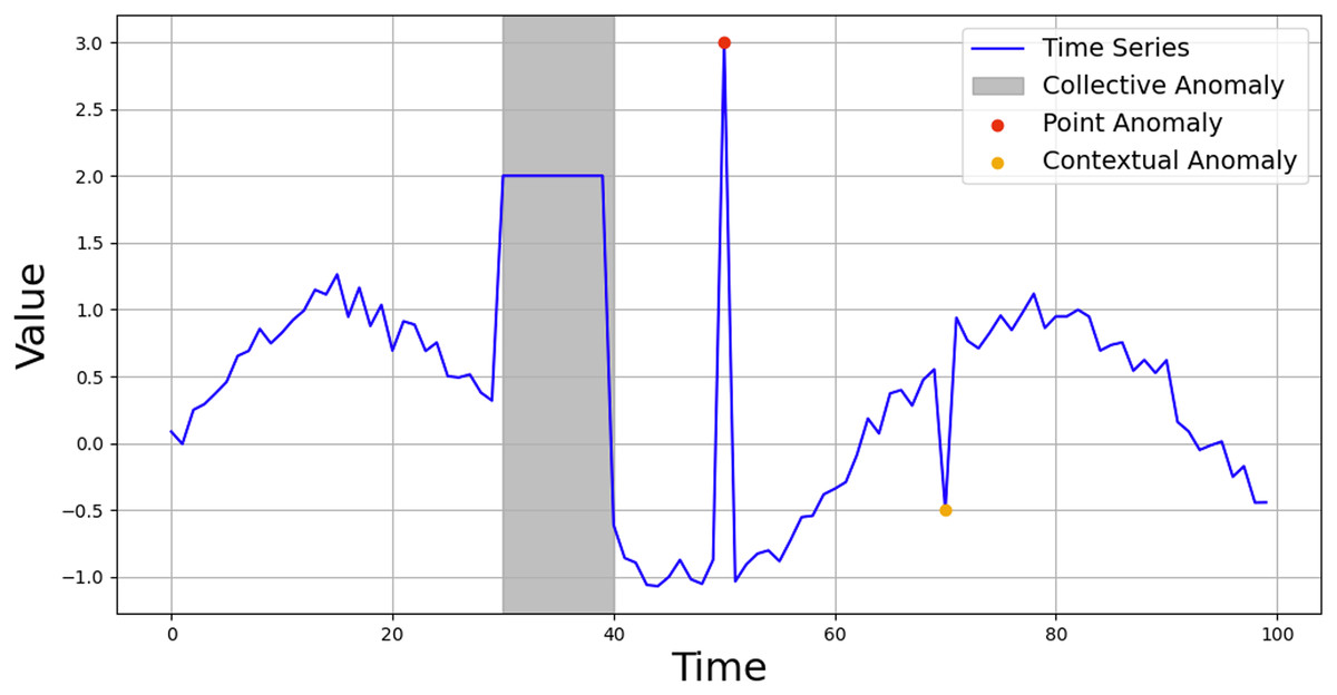
Figure 1: Anomaly types of time series data.
Reproduced from Park & Jang (2024).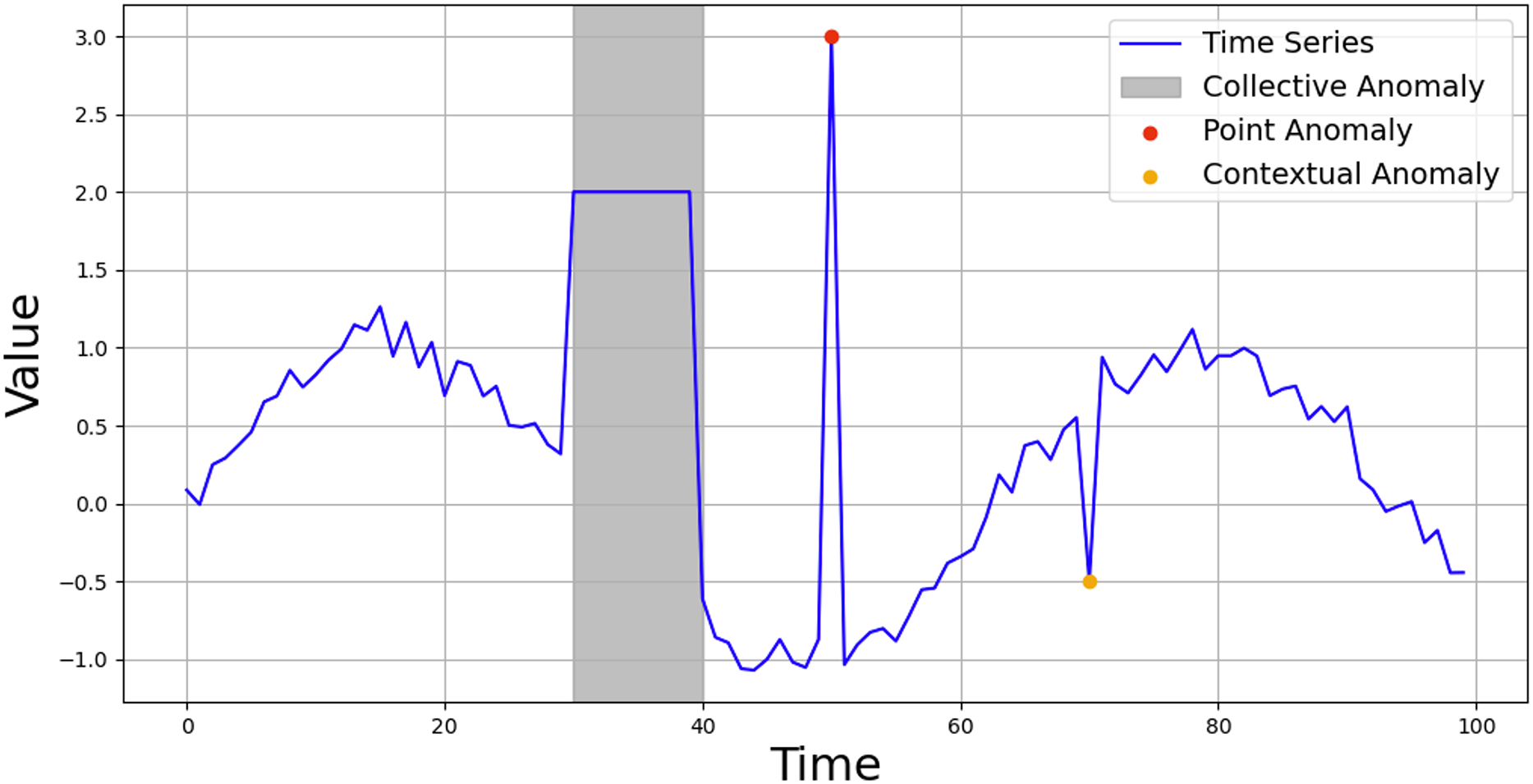
Spiking neural networks
Spiking neural networks (SNNs), also referred to as “third-generation neural networks,” use spikes in the form of pulses instead of digital data to represent the input and output of neurons (Almasri & Sahran, 2014). SNNs have earned considerable attention due to their ability to model the temporal dynamics of data more effectively than traditional neural networks. Their event-driven nature, which only activates neurons upon the receipt of input spikes, allows them to mimic biological neural processes and achieve substantial energy efficiency (Wang et al., 2024). This characteristic makes SNNs particularly suitable for low-power applications such as Internet of Things (IoT) devices and edge computing, where resource constraints and real-time processing are critical (Dan et al., 2024; Lucas & Portillo, 2024).
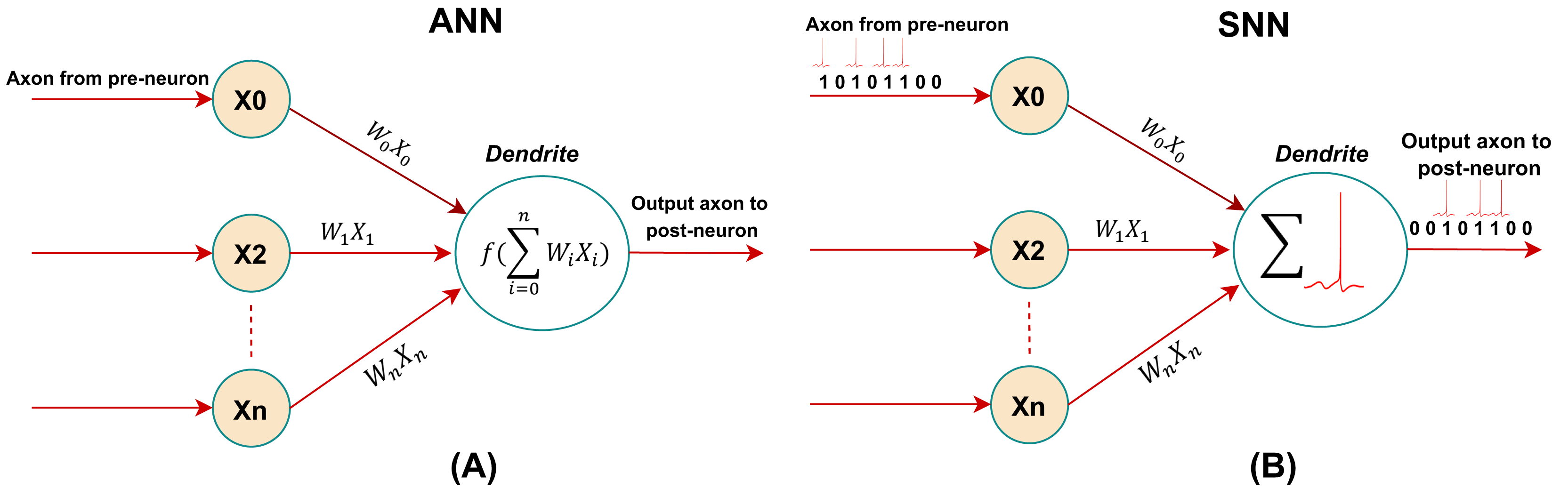
Unlike the neuron models used in artificial neural networks (ANNs), spiking neurons do not operate based on matrix-vector multiplication, but fire spikes when their membrane potential reaches the spiking threshold (Plagwitz et al., 2023). In ANNs, neurons take continuous real-valued inputs and outputs. As illustrated in Fig. 2, derived from Yamazaki et al. (2022), the ANN neurons compute a weighted sum of the input signal, followed by applying a nonlinear activation function to produce the output signal. In contrast, spiking neurons in SNN offer a more detailed and realistic representation of biological neurons. Spiking neurons, similar to their biological counterparts, are connected through synapses, and the membrane potential and activation threshold primarily govern their behavior. The spike signal received by the dendrites alters the membrane potential of the neuron, and once this accumulated potential reaches the threshold, the neuron emits a spike signal from its axon to the next neuron (Wu et al., 2024). Numerous enhancements and variations of the spiking neuron model have been introduced, including the evolving spiking neural network (eSNN), which involves the incremental growth of the number of spiking neurons over time. This gradual evolution allows eSNNs to efficiently capture and interpret temporal patterns from continuous data streams, making them ideal for adaptive learning in real-time scenarios (Maciąg et al., 2021).
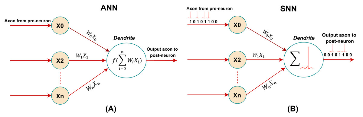
Figure 2: Representation of neuron models: (A) artificial neuron. (B) spiking neuron.
Online evolving spiking neural networks
One of the most promising SNN designs is the evolving spiking neural network (eSNN) (Lobo et al., 2020). By gradually merging the generated neurons to find the pattern in the given issue, the eSNN improves the flexibility of SNN (Kasabov, 2019). To gather clusters and patterns from new data, the spiking neurons in this type of network are created (evolved) and incrementally combined. The eSNN repeatedly generated repositories for every class to provide new data without retraining the learned dataset (Schliebs & Kasabov, 2013). The neural model of eSNN facilitates rapid real-time simulations of large-scale networks with minimal computational overhead. These characteristics position eSNNs as highly suitable for online learning environments (Wysoski, Benuskova & Kasabov, 2006).
Motivated by these advantages, Lobo et al. (2018) further enhanced the eSNN model and developed the Online eSNN (OeSNN) to address the evolving demands of online data processing. OeSNN networks were developed to handle classification tasks in streaming data, building upon the eSNN architecture, which was initially designed for classifying batch data with distinct training and testing phases (Kasabov, 2007). Both eSNN and OeSNN share a similar structure consisting of input and output layers; however, the number of output neurons in OeSNN is limited, whereas eSNN permits an unlimited number of output neurons. This restriction in OeSNN is driven by the demands of classifying data streams, where vast amounts of input data are typically processed, and strict memory limitations must be observed (Maciąg et al., 2021). The OeSNN constructs a repository of output neurons corresponding to training patterns. For each class-specific training pattern, a new output neuron is created and connected to all pre-synaptic neurons in the preceding layer through synaptic weights . The architecture of OeSNN is presented in Fig. 3, adapted from Maciąg et al. (2021).
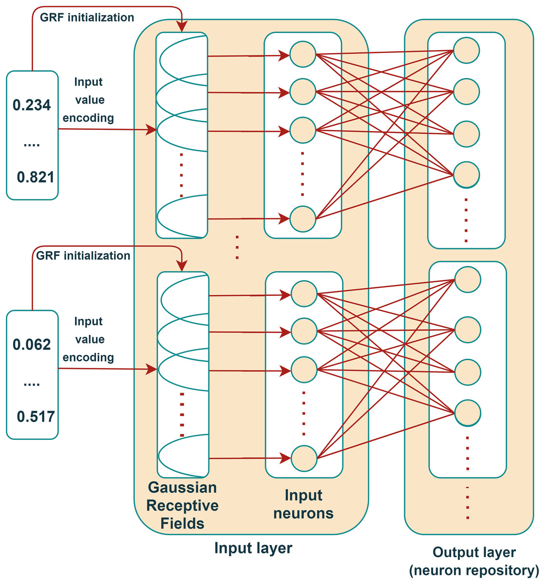
Figure 3: OeSNN architecture.
Reproduced from Maciąg et al. (2021).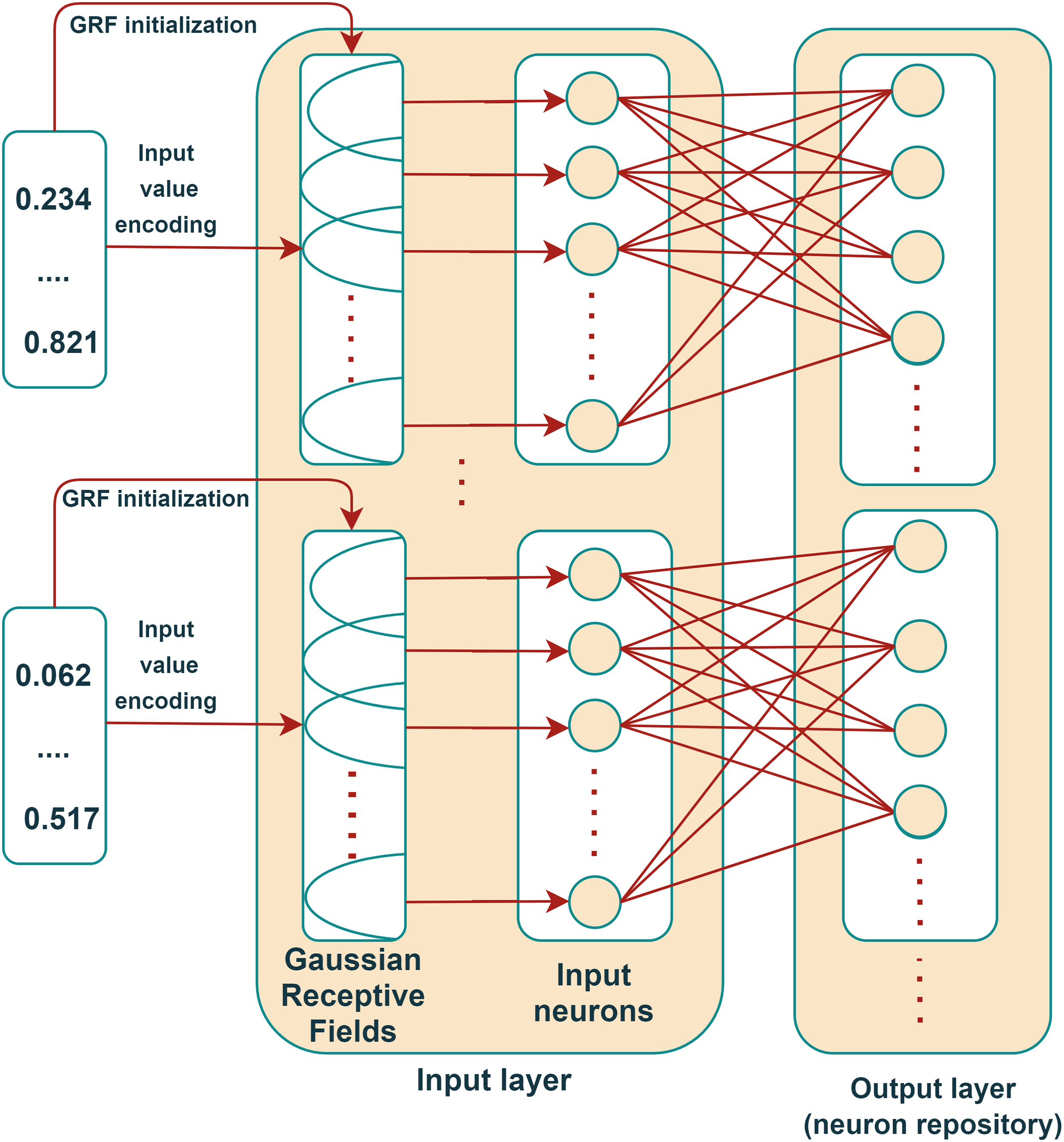
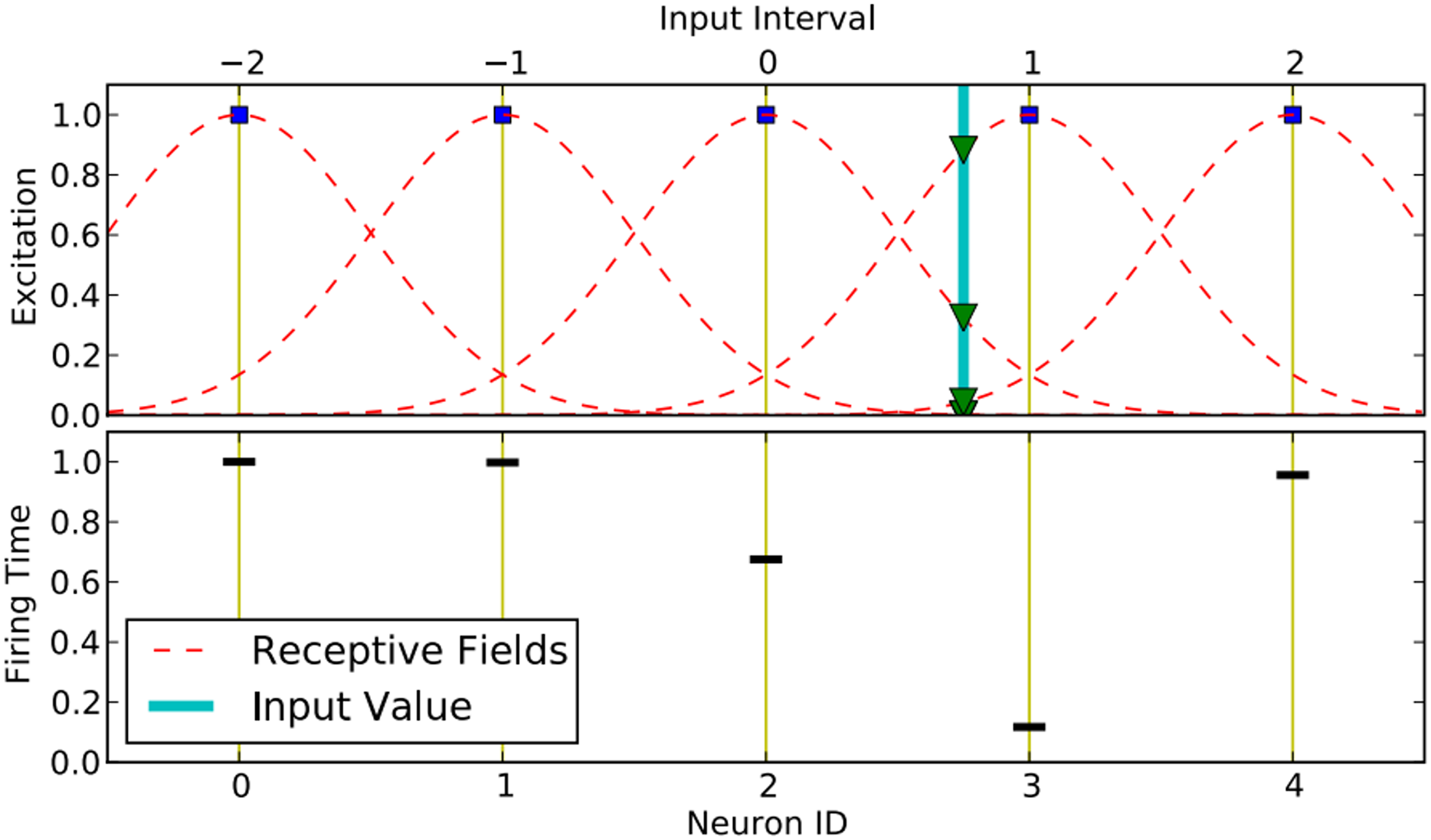
To classify real-valued datasets using OeSNN, data samples are transformed into Spatio-temporal spike patterns using neural encoding techniques. A widely adopted method is the rank-order population encoding, an extension of the rank-order encoding proposed by Thorpe & Gautrais (1998). This technique prioritizes spikes based on their temporal order across synapses, providing additional information to the network, and utilizes the Gaussian Receptive Field (GRF) encoding scheme, as described by Bohte, Kok & La Poutré (2002), which distributes continuous input values across several neurons with overlapping Gaussian activation functions. Each neuron in this scheme fires only once within the coding interval, ensuring a robust representation of input features.
The population encoding based on GRF is explained in Fig. 4, derived from Hamed, Kasabov & Shamsuddin (2011). The intersection points with each Gaussian are calculated (triangles) with an input value v = 0.75 (thick straight line in the top figure). These intersection points are then converted into spike time delays (see the lower figure). During encoding, Gaussian Receptive Field Neurons (GRFNs) are employed to distribute input samples with overlapping sensitivity profiles, ensuring each feature is transformed into a spatio-temporal spike pattern. This approach effectively captures the temporal dynamics of the input data, facilitating precise and robust classification. The center and width of each GRF pre-synaptic neuron are computed as follows:
(1)
(2)
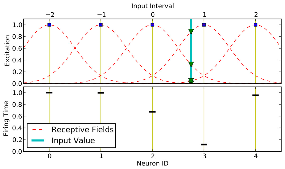
Figure 4: Population encoding based on Gaussian receptive fields.
Here, and representing the interval values of the nth feature in a given window size, is the number of receptive fields (GRF) for each feature. is the overlap factor parameter, which regulates how much Gaussian Random Fields overlap. The output of neuron j is represented as:
(3)
Here x is the input sample, the firing time for each pre-synaptic neuron j is defined as:
(4)
Here, T is the spike interval.
The LIF model is utilized to generate initial neurons. The neuron fires only once and only when the postsynaptic potential (PSP) value is higher than its threshold value. PSP of the ith neuron is identified as:
(5)
Here represents the synaptic weight between pre-synaptic neuron j and output neuron i, while order(j) denotes the firing rank of the pre-synaptic neuron, and mod represents the modulation factor, takes a value within the range [0, 1]. For each training sample belonging to the same class, a new output neuron is created and connected to all pre-synaptic neurons in the preceding layer, with weights assigned based on their rank order as follows:
(6)
The threshold of a newly generated output neuron is defined as:
(7)
Here is a user-fixed value in (0, 1].
The weight vector of a newly produced output neuron is compared with those of existing neurons in the repository. If the Euclidean Distance between the new neuron’s weight vector and that of any existing output neuron is less than or equal to the SIM, the neurons are merged. In this case, the threshold and the weight vector are updated using the following formulas:
(8)
(9)
The variable “M” indicates how many mergers the same output neuron has been involved in during the OeSNN’s learning phase. Following a merger, the model proceeds using the updated neuron representation and discards the weight vector of the newly created neuron. On the other hand, the newly created output neuron is added to the repository if no existing neuron in the repository meets the similarity criteria (based on the SIM value).
Building upon the adaptation of the OeSNN by Lobo et al. (2018), Maciąg et al. (2021) recently introduced the OeSNN-UAD method for detecting anomalies in streaming data. In contrast to the original OeSNN, the OeSNN-UAD operates in an unsupervised manner, without isolating output neurons into distinct groups. Instead, it integrates three additional modules: value correction, anomaly classification, and output value generation for candidate output neurons. The OeSNN-UAD identifies an input as anomalous under two specific conditions: firstly, when no output neurons in the repository are activated, and secondly, when the deviation between the predicted and actual input values exceeds the sum of the prediction error and a user-defined multiple of the recent standard deviation.
Overview of the ABC algorithm
In the present era, the popularity of metaheuristic optimization algorithms has increased exponentially due to their tangible impact on the resolution of optimization problems. Numerous metaheuristic algorithms are inspired by the collective intelligence found in swarms of insects and animals, including ants, whales, lemurs, chimps, and wolves (Abasi et al., 2022). For instance, the proficient swarm intelligence behaviors displayed by honeybees have inspired the development of algorithms for problem-solving and optimization tasks (Hussein, Sahran & Sheikh Abdullah, 2017; Qasem et al., 2022). These algorithms typically start with a set of randomly generated solutions and iteratively improve them using intelligent operators designed to balance exploration and exploitation of the search space. The exploration phase searches to investigate diverse regions of the solution space, while the exploitation phase focuses on refining existing solutions to achieve optimality. By combining these phases and leveraging accumulated knowledge from prior iterations, metaheuristic algorithms have been widely successful in tackling both global and local optimization challenges (Alorf, 2023).
The ABC algorithm is a metaheuristic optimization algorithm inspired by the intelligent foraging behaviors observed in honeybee swarms. It has proven effective in solving a range of optimization issues (Abdullah, Nseef & Turky, 2018; Alrosan et al., 2021). The ABC, first proposed by Karaboga (2005), models the behaviors of three types of bees: employed bees, onlooker bees, and scout bees. The employed bees are responsible for locating food sources and disseminating this information to the onlooker bees via a waggle dance, which conveys the quality and location of the food source. Subsequently, onlookers probabilistically select food sources based on this information, while scout bees explore new areas if a food source becomes unproductive (Hacılar et al., 2024).
Since its introduction in 2005, the ABC algorithm has gained widespread acceptance due to its simplicity, flexibility, and efficiency in solving complex optimization problems, particularly in high-dimensional and multimodal search spaces. One of the key strengths of ABC is its capacity to effectively balance exploration and exploitation through its three bee types, employed, onlooker, and scout bees. This balance prevents the algorithm from becoming trapped in local optima while enabling efficient convergence towards global solutions. In ABC, the food sources represent potential solutions, and the quality of the food source is indicative of the fitness of a solution. The algorithm operates in cycles, whereby solutions are iteratively improved. In each iteration of the algorithm, the employed bees modify the current solution to produce a new one. This is achieved through the application of a greedy selection mechanism, whereby the superior solution is retained. Subsequently, onlooker bees select the superior solutions for further refinement. Suppose a solution fails to improve after a predefined number of attempts. In that case, it is abandoned and the scout bees embark on a random search for new candidate solutions, thereby ensuring diversity within the solution space (Yang et al., 2024).
The ABC algorithm begins by initializing its control parameters. These include the Solutions Number (SN), which represents the population size or the number of potential food sources. Maximum Cycles Number (MCN) is the maximum number of iterations or evaluations that serve as a termination criterion. Limit (abandonment criteria) is the parameter that defines the maximum number of exploitations allowed before a food source is abandoned.
In the first foraging cycle, the scout bees are responsible for discovering new food sources, and they randomly assign initial positions to these food sources using a method Eq. (10), which helps guide this random placement.
(10)
Here, , the value of D represents the dimension of the problem (number of optimization parameters), whereas SN refers to the number of food sources, . The upper and lower boundaries of parameter, respectively.
Each food source is assessed and assigned both a cost function value ( ) and a counter value ( ). The scout bees associated with more profitable food sources transition into employed bees, tasked with exploring the surrounding areas of these sources using Eq. (11) to identify superior alternatives for exploitation:
(11) where k is a randomly selected neighboring index where represents a randomly chosen dimension index, and ∈ [−1,1] is a random number generated from a uniform distribution.
If the newly generated solution proves superior to the current solution , the current solution is replaced, and is reset to zero. Otherwise, the current solution is kept in the population, and is increased by 1.
During the initial cycle, onlooker bees (who were initially scout bees of less profitable solutions) remain in the hive. They select a more profitable food source based on the information provided by the employed bees. This is simulated by assigning a probability to each food source based on the profitability values using Eqs. (12) and (13) and implementing a roulette wheel selection method, in which more bees are likely to be recruited to more profitable sources, and low-quality solutions have a lower chance of being chosen.
(12)
(13) where the is the objective function and the probability of the food source i.
Once an onlooker bee has selected a food source, it proceeds to perform the same search operation as the employed bee, as described by Eq. (11). A greedy selection process is then used to update the counter ( ) associated with the chosen solution. These counters are compared with the predefined limit parameter during the scout bee phase to identify which sources have been sufficiently exploited. If the counter ( exceeds the limit, the corresponding solution is considered exhausted, and a new, previously unexplored solution is generated using Eq. (10) in place of . This sequence of operations is repeated until the termination criterion is met.
Proposed method
In this section, comprehensive details regarding the proposed HABCOeSNN are provided. We extensively investigate the optimization of five key hyperparameters of OeSNN, including window size (Wsize), anomaly classification factor (ε), similarity value (SIM), modulation factor (MOD), and threshold factor (C), to determine the optimal configuration.
To systematically explore the influence of these hyperparameters on anomaly detection accuracy, we employed an attribute evaluation method, the information gain attribute evaluation approach, to identify which hyperparameters had the greatest effect on the performance of the OeSNN.
Based on our previous experiment (Rehan et al., 2025), and the information gain analysis, we grouped the five hyperparameters into three distinct sets. Set 1 includes two hyperparameters, Wsize and ε, selected based on previous experimental findings. Set 2 consists of hyperparameters: SIM, MOD, and C, which were identified by information gain as the most impactful. Finally, Set 3 combines all five hyperparameters to form a comprehensive set. Table 1 provides a detailed breakdown of these groupings.
| Sets | Hyperparameters |
|---|---|
| Set 1 | Wsize and ε. |
| Set 2 | SIM, MOD and C. |
| Set 3 | Wsize, ε, SIM, MOD, and C |
This structured approach enabled a robust and comprehensive investigation of how different combinations of hyperparameters influence OeSNN performance. The candidates, each set of hyperparameters, are randomly initialized, and their performance is continuously refined through iterations. The fitness function, based on the F1-score, guides the search for the optimal hyperparameter values, and the ABC continues updating the candidates until the maximum number of iterations is reached.
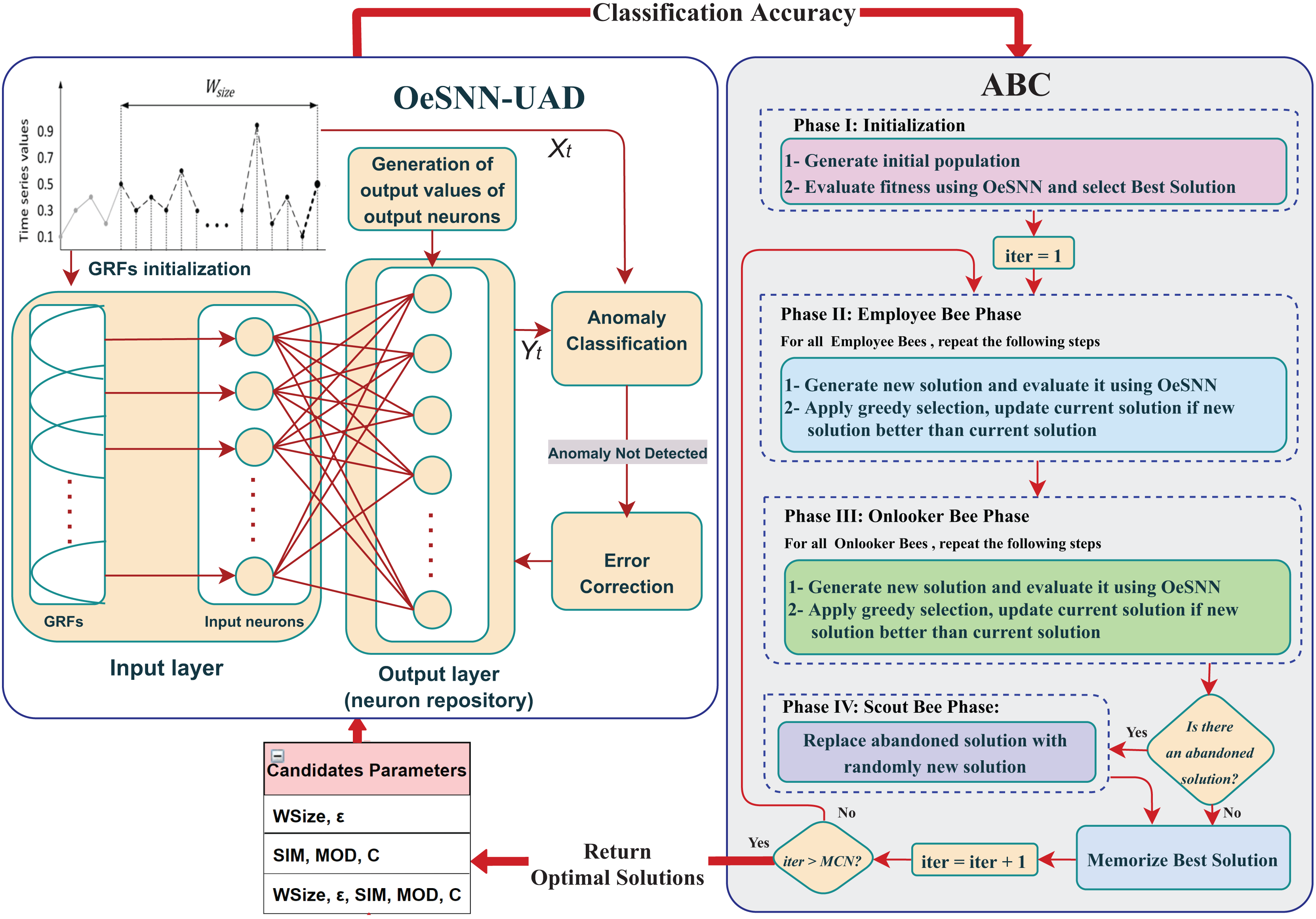
The proposed HABCOeSNN consists of seven main steps that are thoroughly explained below.
Initialization hase
The ABC can be formulated as a 2D matrix where n refers to the number of bees and m refers to the solution size, as expressed in Eq. (14).
(14)
All the candidate solutions (Set 1, Set 2, or Set 3) in the population are randomly initiated from the possible ranges of OeSNN hyperparameters using Eq. (10). Further, the objective function, F1-score, is calculated using OeSNN, and the fitness value for all solutions is evaluated, which gives the initial global Best solution.
Employee bees phase
In this phase, the employee bees generate new candidate solutions using Eq. (11), compute the objective function with the OeSNN, and assess the fitness of each solution using Eq. (12). Then, a greedy selection process is employed to evaluate the newly generated solutions. If the new solution demonstrates an improvement over the existing one, it replaces the current solution; otherwise, no changes are made. This process is repeated for every employee bee in the population to ensure a comprehensive exploration of potential solutions.
Onlooker bees phase
The onlooker phase commences with the calculation of the probability value (P) for each food source obtained from the employed bees by using Eq. (13). Subsequently, a single food source is selected based on its probability value (Pi), resulting in the generation of a new solution by using Eq. (11). The objective function utilizing OeSNN is then calculated, and the fitness value for the novel solution is evaluated using Eq. (12). To assess the efficacy of the new solution, greedy selection is employed. In the event of an enhancement being observed, the new solution is updated with the current solution; conversely, no alterations are made. These procedures are repeated for each onlooker bee within the population.
Scout bees phase
The Scout Bee Phase starts when a food source has not been updated for a specified number of cycles, signaling that the food source has been abandoned. At this point, the abandoned food source is replaced by a randomly chosen one from the search space. The bee previously associated with the abandoned source becomes a scout bee, and a new solution is generated for this scout using Eq. (10).
Memories best solution
Updating and retaining the Best Solution found so far.
Stop criteria
Repeat Steps 2–5 till the termination condition is met.
Return the best solution
These steps will be repeated for each set of the hyperparameters. Furthermore, the results will be thoroughly analyzed to determine the optimal set of hyperparameters. All the above steps of the HABCOeSNN are illustrated as a flowchart in Fig. 5.
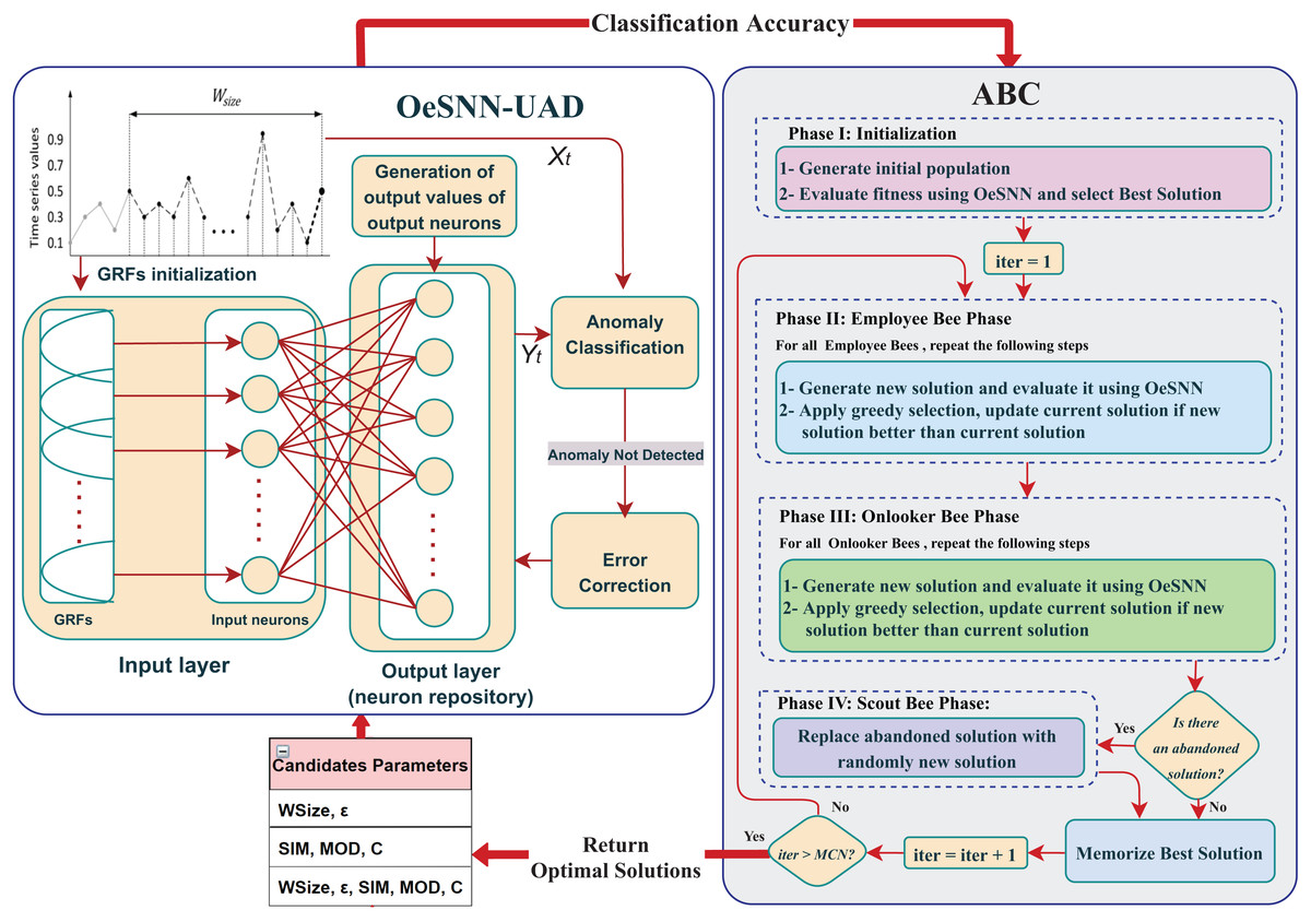
Figure 5: Flowchart of the proposed HABCOeSNN.
The pseudocode of the HABCOeSNN is given below:
| 1. Initialize the ABC parameters: Population size (SN), Maximum Cycles Number (MCN), number of dimensions (D), Lower Bound (lb), Upper Bound (ub), and Maximum number of trials (limit). |
| 2. Initialize the OeSNN parameters: Number of Output Neurons (NOsize), Number of Input Neurons (NIsize), and Output value correction factor (ξ). |
| 3. {------- Generate ABC population -------} |
| 4. |
| 5. Calculate the objective function using OeSNN |
| 6. |
| 7. Set |
| 8. Find the Best Solution in the initial population |
| 9. Set iter = 1 |
| 10. while iter <= MCN do |
| 11. {------- Employee Phase -------} |
| 12. for i = 1 to SN do |
| 13. Select k, where |
| 14. Select j, where |
| 15. |
| 16. Calculate the objective function using OeSNN |
| 17. |
| 18. {---- Apply greedy selection between ----} |
| 19. if ( then |
| 20. |
| 21. |
| 22. else |
| 23. |
| 24. endif |
| 25. end for |
| 26. {------- Calculate the probability P for all solutions ------} |
| 27. |
| 28. {------- OnLooker Phase -------} |
| 29. for i = 1 to SN do |
| 30. {---- Select a food source depending on its probability ----} |
| 31. Select k, where |
| 32. Select j, where |
| 33. |
| 34. Calculate the objective function using OeSNN |
| 35. |
| 36. {---- Apply greedy selection between ----} |
| 37. if ( then |
| 38. |
| 39. |
| 40. else |
| 41. |
| 42. endif |
| 43. end for |
| 44. {------- Scout Phase -------} |
| 45. Set Max_Trial_Index = 0 |
| 46. Set i = 1 |
| 47. while i < SN do |
| 48. if then |
| 49. Max_Trial_Index = i |
| 50. end if |
| 51. i = i + 1 |
| 52. end while |
| 53. if then |
| 54. for j = 1 to D do |
| 55. |
| 56. end for |
| 57. end if |
| 58. Memories the Best Solution |
| 59. iter = iter + 1 |
| 60. end while |
| 61. Return Best Solution |
Results and discussion
The proposed approach is thoroughly evaluated using two well-established benchmark datasets, Yahoo Webscope (Laptev, Amizadeh & Billawala, 2015) and Numenta (Lavin & Ahmad, 2016), which serve as a foundation for assessing the performance of anomaly detection systems. Experiments utilize both synthetic and real-time series data from a variety of domains. The primary objective of this evaluation is to determine the extent to which the proposed method improves the learning capabilities of the OeSNN. During this process, the proposed method is compared with 14 anomaly detection algorithms from the literature. Furthermore, the efficacy of the proposed approach is evaluated against five successful optimization algorithms alongside a range of other classifiers. This comparative analysis aims to highlight the superiority of the proposed HABCOeSNN method in enhancing OeSNN performance and improving accuracy in anomaly detection tasks.
Experimental setup
For the experiments, all evaluation was carried out on a PC with an 11th Gen Intel(R) Core™ i5-11260H processor at 2.60 GHz and 16 GB of RAM, running Windows 11 64-bit. The programming language used for the experiments is Dev C++ 6.3.
Evaluation measures
To assess the performance of HABCOeSNN in the anomaly detection task, multiple evaluation metrics are employed to offer a well-rounded perspective, particularly in handling imbalanced datasets:
Precision
Precision measures the proportion of true anomalies (true positives, TP) out of all detected anomalies (TP + false positives, FP). It emphasizes reducing false positives, and its formula is:
(15)
Recall
Recall reflects the proportion of correctly identified anomalies from the total actual anomalies (true positives, TP, and false negatives, FN), highlighting the model’s ability to detect all anomalies:
(16)
F1-score
The F1-score is the harmonic mean of precision and recall, balancing the trade-off between them:
(17)
Balanced accuracy (BA)
Balanced accuracy (BA) considers both sensitivity (recall) and specificity, providing a more balanced measure, especially useful in imbalanced datasets:
(18)
Matthew’s correlation coefficient (MCC)
Matthew’s correlation coefficient (MCC) evaluates the model’s performance across all four confusion matrix outcomes: true positives (TP), true negatives (TN), false positives (FP), and false negatives (FN). It is particularly suited for imbalanced data:
(19)
Parameters setting
Before the experiment, the ABC and OeSNN parameters were established. According to research on the ABC algorithm, it is observed that increasing the colony size generally leads to better performance. However, after reaching a certain threshold, further increasing the colony size does not yield significant improvements in the algorithm’s performance (Karaboga & Basturk, 2008). The conducted experiments on different test problems recommended that a colony size of 50 to 100 is sufficient to achieve acceptable convergence without unnecessarily increasing computational costs. Table 2 lists the ABC parameters that established before the experimental conditions and were derived from Karaboga & Basturk (2008). The setting of the hyperparameter values for OeSNN is provided based on the works of Kasabov et al. (2014), Tu, Kasabov & Yang (2017), and Maciąg et al. (2021), as shown in Table 3.
| Parameters | Initialization values |
|---|---|
| Colony size (CS) | 50 |
| Employee bees | 25 |
| Onlooker bees | 25 |
| Scout bee | 1 |
| Trials limit | 0.6 * CS * Dimension |
| Max iteration | 100 |
| Parameter | Description | Value |
|---|---|---|
| NIsize | Input neurons | 10 |
| NOsize | Output neurons | 50 |
| SIM | Similarity value | (0, 1] |
| MOD | Modulation factor | (0, 1) |
| C | Fire threshold fraction | (0, 1] |
| ξ | Error correction factor | 0.9 |
| Wsize | Input window size | [100–600] |
| ε | Anomaly classification factor | [2–7] |
Experimental I: anomaly detection in the Yahoo Webscope dataset
Dataset description
The Yahoo Webscope dataset is divided into four sub-benchmarks: A1, A2, A3, and A4, comprising 367 time series, both real and synthetic, with data points ranging from 1,420 to 1,680. These series have hourly time-stamps, and anomalies were manually identified based on the Yahoo S5 guidelines. The A1Benchmark contains 67 real datasets of Yahoo login activity, while the A2Benchmark and A3Benchmark each include 100 synthetic datasets with single anomalies, whereas the A3Benchmark adds features such as trends, noise, and seasonality. The A4Benchmark comprises 100 synthetic datasets, where anomalies arise from abrupt shifts in data trends. Across all benchmarks, the time series are highly imbalanced, with anomalies accounting for less than 1% of the input data (Maciąg et al., 2021). Table 4 presents the properties of these datasets, which include the total number of data files, the total number of anomalies in each category, and the total number of observations.
| Categories | Time series | Total anomalies | Total instances |
|---|---|---|---|
| A1Benchmark | real_1–ral67 | 1,669 | 94,866 |
| A2Benchmark | Synthetic_1–Synthetic_100 | 466 | 142,100 |
| A3Benchmark | TS 1–TS 100 | 943 | 168,000 |
| A4Benchmark | TS 1–TS 100 | 837 | 168,000 |
Results
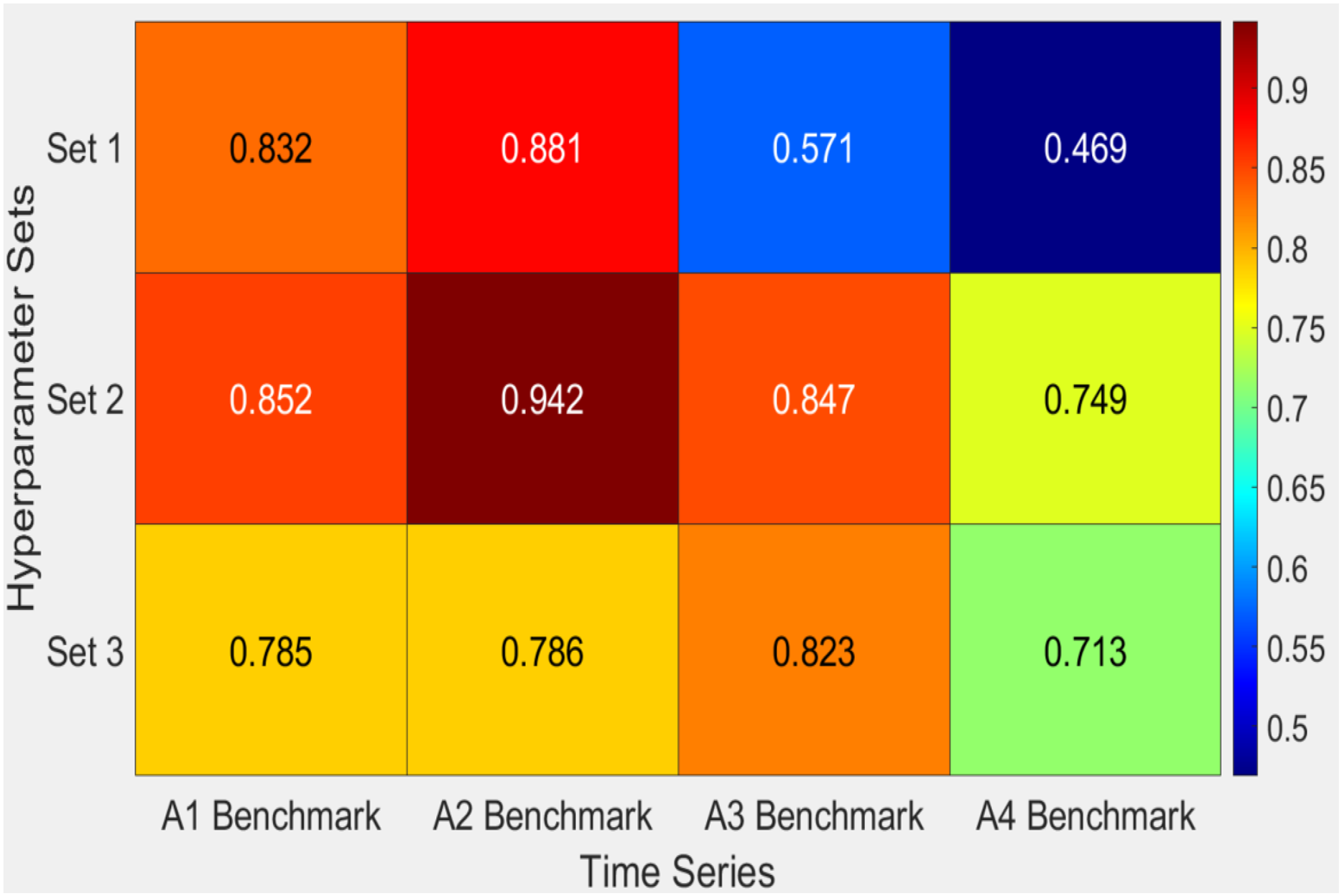
The findings shown in Table 5 and the heatmap analysis in Fig. 6 highlight the differences in performance between the three sets of hyperparameters (Sets 1, Set 2, and Set 3) when applied to different benchmark datasets. Set 2 proves to be the most efficient configuration, achieving the most excellent F1 scores across the majority of datasets, including A2Benchmark with a value of 0.942 and A1Benchmark with 0.852. This demonstrates the resilience of the proposed HABCOeSNN in detecting anomalies, striking a balance between precision and recall. Although Set 3 has competitive recall values, especially in A2Benchmark, its lower F1 scores, as seen in A4Benchmark with a value of 0.713, indicate compromises between precision and recall. Regarding Set 1, it is noticeably less flexible in most datasets but produces excellent outcomes in some situations, as indicated by its lower F1 scores in A3Benchmark (0.571) and A4Benchmark (0.469). These variations in performance are influenced by the inherent characteristics of the datasets, which include both real and synthetic time series. Overall, Set 2 demonstrates the most balanced and robust performance across diverse datasets.
| Categories | Set 1 | Set 2 | Set 3 | ||||||||||||
|---|---|---|---|---|---|---|---|---|---|---|---|---|---|---|---|
| Prec. | Rec. | F1 | BA | MCC | Prec. | Rec. | F1 | BA | MCC | Prec. | Rec. | F1 | BA | MCC | |
| A1Benchmark | 0.876 | 0.828 | 0.832 | 0.911 | 0.838 | 0.872 | 0.886 | 0.852 | 0.938 | 0.861 | 0.761 | 0.901 | 0.785 | 0.946 | 0.803 |
| A2Benchmark | 0.910 | 0.934 | 0.881 | 0.966 | 0.895 | 0.938 | 0.997 | 0.942 | 0.998 | 0.951 | 0.770 | 0.995 | 0.786 | 0.990 | 0.812 |
| A3Benchmark | 0.826 | 0.477 | 0.571 | 0.738 | 0.606 | 0.968 | 0.770 | 0.847 | 0.885 | 0.857 | 0.958 | 0.743 | 0.823 | 0.871 | 0.836 |
| A4Benchmark | 0.668 | 0.450 | 0.469 | 0.724 | 0.505 | 0.894 | 0.680 | 0.749 | 0.840 | 0.766 | 0.883 | 0.638 | 0.713 | 0.819 | 0.734 |
Note:
The bold numbers indicate the best results.
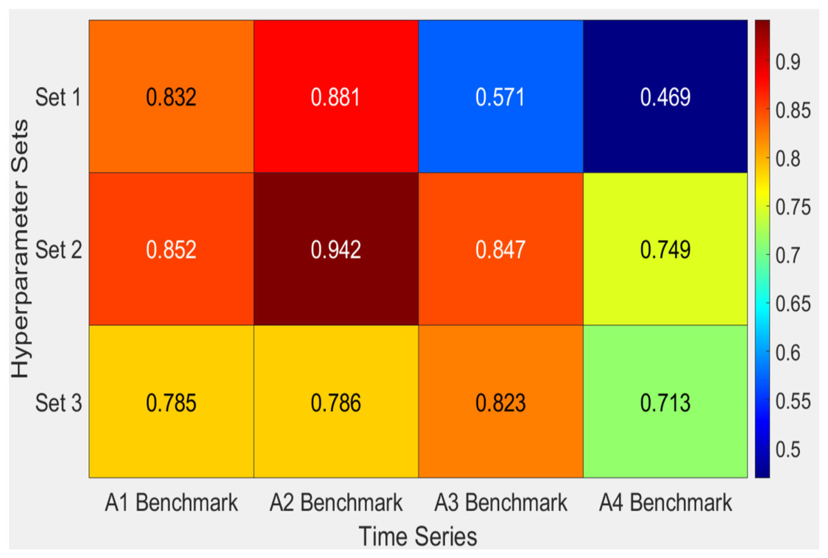
Figure 6: Heatmap of F1-score obtained by the HABCOeSNN for sets of hyperparameters on the Yahoo dataset.
Moreover, to evaluate the performance of hyperparameter sets comprehensively across multiple time series, a complementary Multi-Criteria Decision Making (MCDM) approach was employed, integrating the Weighted Sum Model (WSM) and the Technique for Order Preference by Similarity to Ideal Solution (TOPSIS). Table 6 shows the evaluation of the performance of the hyperparameters: Set 1, Set 2, and Set 3. Set 2 consistently emerges as the best-performing configuration, achieving the highest scores in the WSM score (e.g., 0.888 in A1Benchmark and 0.967 in A2Benchmark) and being ranked first across all datasets in TOPSIS, indicating its robustness and balance across evaluation metrics. Set 1 performs competitively in some cases, such as a WSM score of 0.921 in A2Benchmark, but is generally ranked second, reflecting slightly less optimization than Set 2. Set 3 exhibits variability, with strong performance in A3Benchmark and A4Benchmark, but lower rankings in A1Benchmark and A2Benchmark, indicating inconsistent results across datasets. Overall, Set 2 demonstrates the most balanced and reliable performance, making it the optimal configuration for these benchmarks.
| Categories | Weighted sum scores | TOPSIS ranks | ||||
|---|---|---|---|---|---|---|
| Set 1 | Set 2 | Set 3 | Set 1 | Set 2 | Set 3 | |
| A1Benchmark | 0.864 | 0.888 | 0.848 | 2 | 1 | 3 |
| A2Benchmark | 0.921 | 0.967 | 0.878 | 2 | 1 | 3 |
| A3Benchmark | 0.660 | 0.872 | 0.853 | 3 | 1 | 2 |
| A4Benchmark | 0.585 | 0.796 | 0.769 | 3 | 1 | 2 |
Note:
The bold numbers indicate the best results.
Table 7 presents a comparative analysis of various anomaly detection methods across four benchmark datasets (A1Benchmark to A4Benchmark), focusing on the performance of HABCOeSNN. The proposed method utilizing Set 2 demonstrates superior effectiveness, consistently outperforming competing techniques. In particular, HABCOeSNN surpasses popular methods such as Twitter Anomaly and Yahoo EGADS on the A1, A2, and A4 benchmarks, achieving F1-scores of 0.852, 0.942, and 0.749, respectively. Although DeepAnT performs well in the A3Benchmark, the proposed HABCOeSNN with Set 2 consistently succeeds across all datasets.
| Categories | Yahoo EGADS1 | Twitter Anomaly1 | DeepAnT1 | OeSNN-UAD2 | OeSNN-D3 | Set 1 | Set 2 | Set 3 |
|---|---|---|---|---|---|---|---|---|
| A1Benchmark | 0.470 | 0.470 | 0.460 | 0.700 | 0.405 | 0.832 | 0.852 | 0.785 |
| A2Benchmark | 0.580 | 0.000 | 0.940 | 0.690 | 0.451 | 0.881 | 0.942 | 0.786 |
| A3Benchmark | 0.480 | 0.300 | 0.870 | 0.410 | 0.110 | 0.571 | 0.847 | 0.823 |
| A4Benchmark | 0.290 | 0.340 | 0.680 | 0.340 | 0.147 | 0.469 | 0.749 | 0.713 |
Notes:
The bold numbers indicate the best results.
Performance comparison with other classifiers
Table 8 shows a comparison of the HABCOeSNN model against three widely recognized classifiers, Random Forest (RF), Support Vector Machine (SVM), and k-Nearest Neighbors (kNN), as presented in Sina & Thomas (2019). The results indicate that HABCOeSNN consistently outperforms these conventional machine learning techniques across all four Yahoo Webscope benchmarks, regardless of the hyperparameter set used. Set 2 achieves an impressive F1-score across all datasets, underscoring the model’s intense precision and effectiveness in identifying anomalies with minimal false positives.
| Categories | Measure | Random forest* | SVM* | kNN* | Set 1 | Set 2 | Set 3 |
|---|---|---|---|---|---|---|---|
| A1Benchmark | Precision | 0.40 | 0.46 | 0.44 | 0.88 | 0.87 | 0.76 |
| Recall | 0.77 | 0.76 | 0.76 | 0.83 | 0.89 | 0.90 | |
| F1-score | 0.52 | 0.58 | 0.56 | 0.83 | 0.85 | 0.76 | |
| A2Benchmark | Precision | 0.48 | 0.82 | 0.48 | 0.91 | 0.94 | 0.77 |
| Recall | 0.98 | 0.98 | 0.98 | 0.93 | 0.997 | 0.995 | |
| F1-score | 0.65 | 0.90 | 0.65 | 0.88 | 0.94 | 0.79 | |
| A3Benchmark | Precision | 0.84 | 0.83 | 0.87 | 0.83 | 0.97 | 0.96 |
| Recall | 0.69 | 0.64 | 0.68 | 0.48 | 0.77 | 0.74 | |
| F1-score | 0.75 | 0.72 | 0.76 | 0.57 | 0.85 | 0.82 | |
| A4Benchmark | Precision | 0.69 | 0.71 | 0.68 | 0.67 | 0.89 | 0.88 |
| Recall | 0.61 | 0.61 | 0.59 | 0.45 | 0.68 | 0.64 | |
| F1-score | 0.65 | 0.66 | 0.63 | 0.47 | 0.75 | 0.71 |
Additionally, we employ the MCDM approach to evaluate the performance of the HABCOeSNN across different classifiers. The results reported in Table 9 demonstrate that Set 2 consistently exhibits superior performance compared to other classifiers on the A1–A4 benchmarks, with the highest scores (0.866, 0.955, 0.858, and 0.768, respectively). The findings demonstrate that Set 2 consistently outperforms other classifiers in TOPSIS rankings, occupying the top position across all benchmarks. This outcome reflects the superior and balanced performance of Set 2, as evaluated using a multi-criteria approach. Although models such as SVM and kNN demonstrate efficacy, their inconsistencies across benchmarks highlight the superiority of Set 2 in terms of reliability and effectiveness. The TOPSIS rankings, which emphasize proximity to the optimal solution, reinforce the capacity of Set 2 to deliver optimal results, thereby establishing it as the most reliable approach for the given benchmarks.
| Categories | Weighted sum scores | TOPSIS ranks | ||||||
|---|---|---|---|---|---|---|---|---|
| Random forest | SVM | kNN | Set 2 | Random forest | SVM | kNN | Set 2 | |
| A1Benchmark | 0.553 | 0.595 | 0.580 | 0.866 | 4 | 2 | 3 | 1 |
| A2Benchmark | 0.690 | 0.900 | 0.690 | 0.955 | 4 | 2 | 3 | 1 |
| A3Benchmark | 0.758 | 0.728 | 0.768 | 0.858 | 3 | 4 | 2 | 1 |
| A4Benchmark | 0.650 | 0.660 | 0.633 | 0.768 | 3 | 2 | 4 | 1 |
Note:
The bold numbers indicate the best results.
Comparative analysis with other optimization algorithms
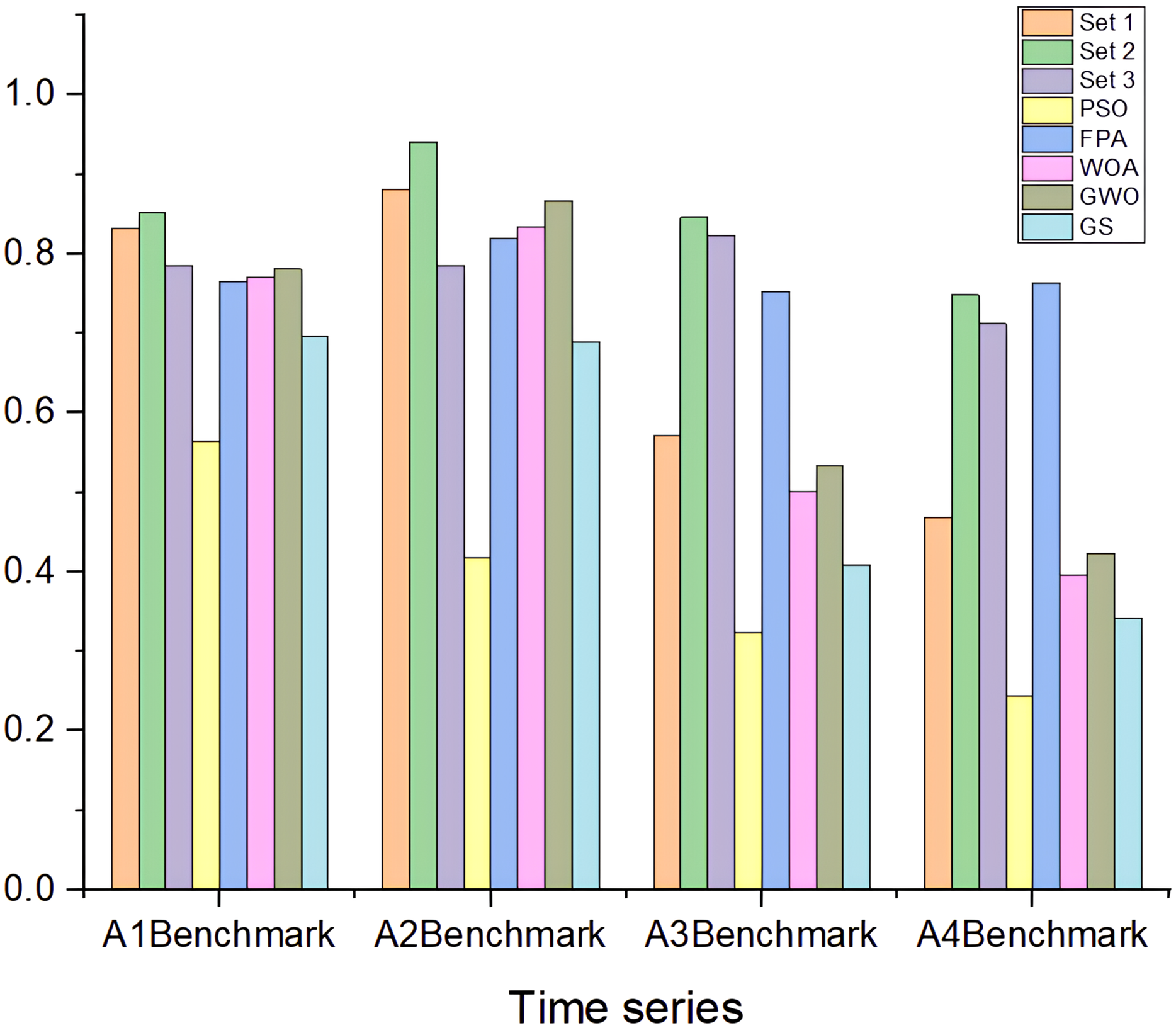
Figure 7 illustrates the comparative performance of the HABCOeSNN model against several optimization algorithms, including PSO, GWO, FPA, WOA, and GS, using three distinct sets of hyperparameters (Sets 1, Set 2, and Set 3). The results indicate that HABCOeSNN with Set 2 consistently achieves the highest overall performance across benchmarks. Set 3 demonstrates strong results in the A3Benchmark, while Set 1 excels in the A1 and A2Benchmarks. In contrast, the PSO and FPA algorithms exhibit varying degrees of success, with PSO performing well in A1 and A2 benchmarks. However, WOA, GWO, and GS perform poorly, particularly in the more complex A3 and A4 benchmarks. These findings highlight the robustness of HABCOeSNN, particularly when optimized with Set 2 hyperparameters across diverse datasets.
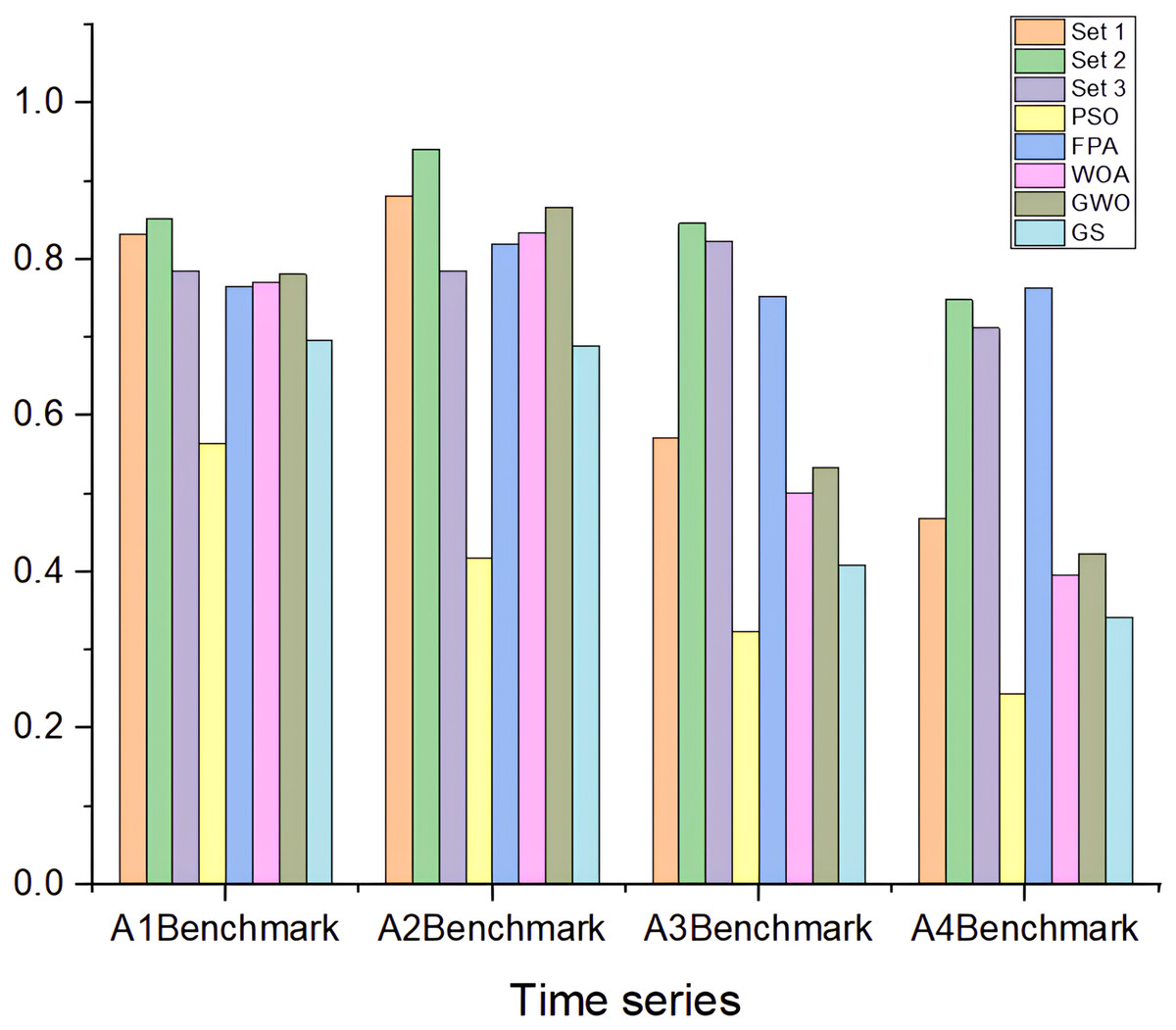
Figure 7: F1-score of HABCOeSNN against PSO, GWO, FPA, WOA, and GS optimization algorithms on Yahoo Webscope dataset.
Experimental II: anomaly detection in the NAB dataset
Dataset description
The NAB dataset comprises seven labeled sub-datasets, six of which contain anomalies, while one contains only normal data and was excluded from the experiments. These sub-datasets include 58 univariate time series with varying lengths, ranging from 1,000 to 22,000 instances. Each series is time-stamped, and the anomaly labels are stored separately. The time series exhibits diverse characteristics, including temporal noise, periodic patterns of varying duration, and concept drift. The data originates from various sources, including online ad click logs, AWS server metrics, and real-world datasets such as hourly NYC taxi schedules, CPU usage, and freeway traffic data (speed or travel time).
Additionally, the dataset includes synthetic data designed to test for anomalous behaviors. Notably, the dataset is imbalanced, with anomalies comprising less than 10% of the data. Additionally, each record in the dataset contains two data items: a time stamp and a value. Table 10 provides more specific details regarding NAB (Xie, Tao & Zeng, 2023).
| Categories | Time series | No. of anomalies | Total instances |
|---|---|---|---|
| ArtificialWith Anomaly | art daily flatmiddle | 403 | 4,032 |
| art daily jumpsdown | 403 | 4,032 | |
| art daily jumpsup | 403 | 4,032 | |
| art daily nojump | 403 | 4,032 | |
| art increase spike density | 403 | 4,032 | |
| art load balancer spikes | 403 | 4,032 | |
| Real Ad exchange | exchange-2 cpc results | 163 | 4,032 |
| exchange-2 cpm results | 162 | 4,032 | |
| exchange-3 cpc results | 153 | 4,032 | |
| exchange-3 cpm results | 153 | 4,032 | |
| exchange-4 cpc results | 165 | 4,032 | |
| exchange-4 cpm results | 164 | 4,032 | |
| Real AWS cloud watch | ec2_cpu utilization_5f5533 | 402 | 4,032 |
| ec2 cpu utilization 24ae8d | 402 | 4,032 | |
| ec2 cpu utilization 53ea38 | 402 | 4,032 | |
| ec2 cpu utilization 77c1ca | 403 | 4,032 | |
| ec2 cpu utilization 825cc2 | 343 | 4,032 | |
| ec2 cpu utilization ac20cd | 403 | 4,032 | |
| ec2 cpu utilization c6585a | 0 | 4,032 | |
| ec2 cpu utilization fe7f93 | 405 | 4,032 | |
| ec2 disk write_bytes 1ef3de | 473 | 4,730 | |
| ec2 disk write_bytes c0d644 | 405 | 4,032 | |
| ec2 network in 5abac7 | 474 | 4,730 | |
| ec2 network in 257a54 | 403 | 4,032 | |
| elb request count8c0756 | 402 | 4,032 | |
| grok asg anomaly | 465 | 4,621 | |
| iio us-east-1 i-a2eb1cd9 NetworkIn | 126 | 1,243 | |
| rds cpu utilization cc0c53 | 402 | 4,032 | |
| rds cpu utilization e47b3b | 402 | 4,032 | |
| Real known cause | ambient temperature system failure | 726 | 7,267 |
| cpu utilization asg misconfiguration | 1,499 | 18,050 | |
| ec2 request latency system failure | 346 | 4,032 | |
| machine temperature system failure | 2,268 | 22,695 | |
| nyc taxi | 1,035 | 10,320 | |
| rogue agent key hold | 190 | 1,882 | |
| rogue agent key updown | 530 | 5,315 | |
| Real traffic | occupancy 6005 | 239 | 2,380 |
| occupancy t4013 | 250 | 2,500 | |
| speed 6005 | 239 | 2,500 | |
| speed 7578 | 116 | 1,127 | |
| speed t4013 | 250 | 2,495 | |
| travel Time 387 | 249 | 2,500 | |
| travel Time 451 | 217 | 2,162 | |
| Real tweets | twitter volume AAPL | 1,588 | 15,902 |
| twitter volume AMZN | 1,580 | 15,831 | |
| twitter volume CRM | 1,593 | 15,902 | |
| twitter volume CVS | 1,526 | 15,853 | |
| twitter volume FB | 1,582 | 15,833 | |
| twitter volume GOOG | 1,432 | 15,842 | |
| twitter volume IBM | 1,590 | 15,893 | |
| twitter volume KO | 1,587 | 15,851 | |
| twitter volume PFE | 1,588 | 15,858 | |
| twitter volume UPS | 1,585 | 15,866 |
Results
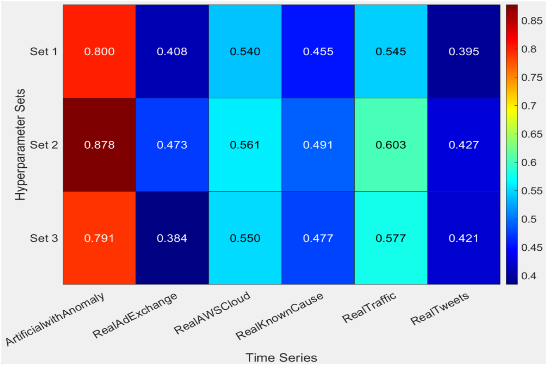
The results presented in Table 11, accompanied by the heatmap visualization in Fig. 8, underscore the superior performance of the HABCOeSNN when employing the Set 2 hyperparameter configuration. Across the time series in the NAB dataset, Set 2 consistently achieves the highest F1-scores, particularly excelling in ArtificialWithAnomaly and RealTraffic, with an F1-score of 0.878 and a Balanced Accuracy (BA) of 0.940. This highlights its capability to balance precision and recall effectively, which is critical for robust anomaly detection. In contrast, Set 1 serves as a baseline with modest performance, while Set 3 exhibits inconsistent results across datasets despite performing well in specific scenarios. Besides, the heatmap clearly illustrates the robustness and adaptability of the HABCOeSNN, reinforcing its role as the optimal configuration for diverse anomaly detection tasks in dynamic streaming environments. Also, the efficacy of various hyperparameter configurations was analyzed across multiple time series using MCDM approaches, including WSM and TOPSIS. According to Table 12, Set 2 is consistently the best arrangement, particularly with datasets such as ArtificialWithAnomaly and RealAdExchange.
| Categories | Set 1 | Set 2 | Set 3 | ||||||||||||
|---|---|---|---|---|---|---|---|---|---|---|---|---|---|---|---|
| Prec. | Rec. | F1 | BA | MCC | Prec. | Rec. | F1 | BA | MCC | Prec. | Rec. | F1 | BA | MCC | |
| ArtificialWithAnomaly | 0.758 | 0.877 | 0.800 | 0.921 | 0.790 | 0.867 | 0.896 | 0.878 | 0.940 | 0.867 | 0.864 | 0.769 | 0.791 | 0.877 | 0.786 |
| RealAdExchange | 0.414 | 0.529 | 0.408 | 0.706 | 0.370 | 0.476 | 0.503 | 0.473 | 0.712 | 0.417 | 0.479 | 0.411 | 0.384 | 0.671 | 0.358 |
| RealAWSCloudwatch | 0.523 | 0.674 | 0.540 | 0.783 | 0.508 | 0.488 | 0.715 | 0.561 | 0.811 | 0.526 | 0.528 | 0.673 | 0.550 | 0.787 | 0.517 |
| RealKnownCause | 0.443 | 0.534 | 0.455 | 0.727 | 0.413 | 0.463 | 0.601 | 0.491 | 0.759 | 0.456 | 0.428 | 0.600 | 0.477 | 0.751 | 0.432 |
| RealTraffic | 0.541 | 0.616 | 0.545 | 0.776 | 0.513 | 0.620 | 0.630 | 0.603 | 0.790 | 0.571 | 0.632 | 0.590 | 0.577 | 0.772 | 0.553 |
| RealTweets | 0.321 | 0.587 | 0.395 | 0.712 | 0.334 | 0.372 | 0.561 | 0.427 | 0.724 | 0.374 | 0.362 | 0.569 | 0.421 | 0.721 | 0.365 |
Note:
The bold numbers indicate the best results.
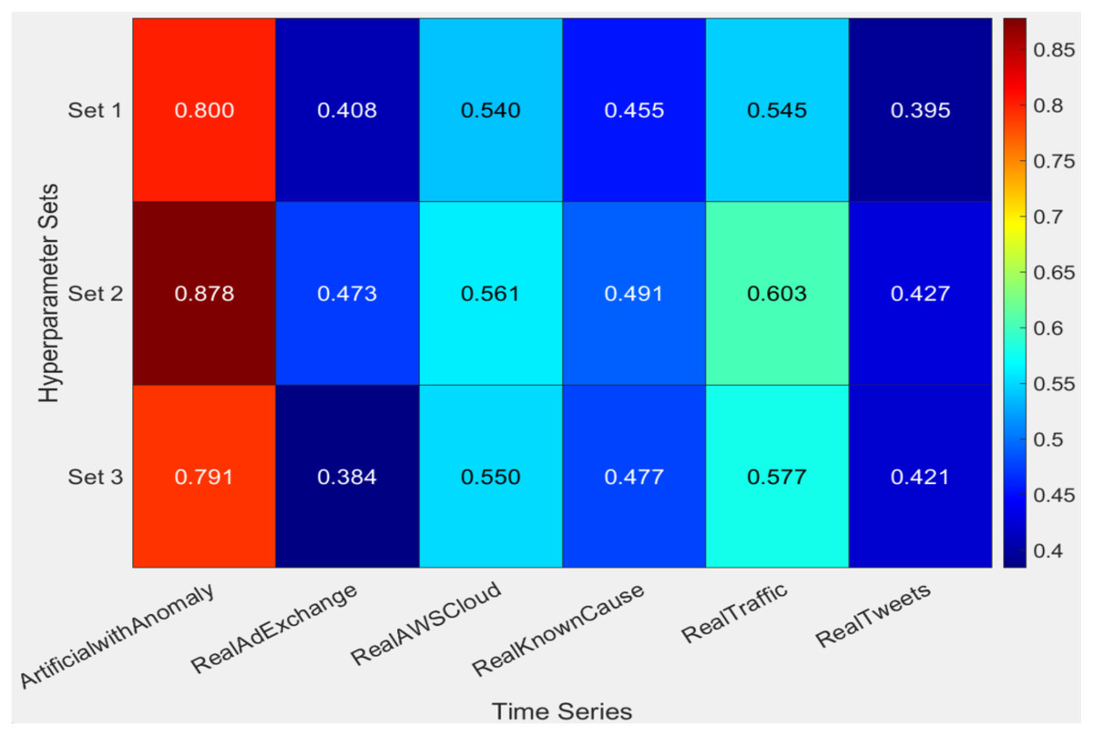
Figure 8: Heatmap of F1-score obtained by the HABCOeSNN regarding the hyperparameters on the NAB dataset.
| Time series | Weighted sum scores | TOPSIS ranks | ||||
|---|---|---|---|---|---|---|
| Set 1 | Set 2 | Set 3 | Set 1 | Set 2 | Set 3 | |
| ArtificialWithAnomaly | 0.841 | 0.897 | 0.818 | 2 | 1 | 3 |
| RealAdExchange | 0.521 | 0.551 | 0.463 | 2 | 1 | 3 |
| RealAWSCloudwatch | 0.633 | 0.647 | 0.614 | 3 | 1 | 2 |
| RealKnownCause | 0.548 | 0.585 | 0.542 | 3 | 1 | 2 |
| RealTraffic | 0.626 | 0.667 | 0.627 | 3 | 1 | 2 |
| RealTweets | 0.509 | 0.528 | 0.493 | 3 | 1 | 2 |
Note:
The bold numbers indicate the best results.
To further assess the HABCOeSNN approach, its performance is compared with that of the state-of-the-art detectors described in Maciąg et al. (2021). Table 13 indicates that Set 2 consistently outperforms the other sets across multiple time series datasets. Specifically, Set 2 exhibits superior performance in the RealAWSCloudwatch and RealKnownCause time series, with consistently higher precision, recall, and balanced accuracy. While Set 3 also produces competitive results, particularly in the RealKnownCause and RealTraffic time series, Set 2 remains the most robust. Its resilience in anomaly detection tasks, demonstrated by consistent performance across all key metrics, provides strong evidence that Set 2 is the most reliable and effective hyperparameter configuration for HABCOeSNN.
| Time series | Bayesian changepoint | Context OSE | EXPoSE | HTM JAVA | KNN CAD | Numenta | NumentaTM | Relative entropy | Skyline | Twitter ADVec | Windowed Gaussian | DeepAnT | OeSNN-UAD | Set 1 | Set 2 | Set 3 |
|---|---|---|---|---|---|---|---|---|---|---|---|---|---|---|---|---|
| ArtificialWithAnomaly | 0.009 | 0.004 | 0.004 | 0.017 | 0.003 | 0.012 | 0.017 | 0.021 | 0.043 | 0.017 | 0.013 | 0.156 | 0.427 | 0.800 | 0.878 | 0.791 |
| RealAdExchange | 0.018 | 0.022 | 0.005 | 0.034 | 0.024 | 0.040 | 0.035 | 0.024 | 0.005 | 0.018 | 0.026 | 0.132 | 0.234 | 0.408 | 0.473 | 0.384 |
| RealAWSCloudwatch | 0.006 | 0.007 | 0.015 | 0.018 | 0.006 | 0.017 | 0.018 | 0.018 | 0.053 | 0.013 | 0.060 | 0.146 | 0.342 | 0.540 | 0.561 | 0.550 |
| RealKnownCause | 0.007 | 0.005 | 0.005 | 0.013 | 0.008 | 0.015 | 0.012 | 0.013 | 0.008 | 0.017 | 0.006 | 0.200 | 0.324 | 0.455 | 0.491 | 0.477 |
| RealTraffic | 0.012 | 0.020 | 0.011 | 0.032 | 0.013 | 0.033 | 0.036 | 0.033 | 0.091 | 0.020 | 0.045 | 0.223 | 0.340 | 0.545 | 0.603 | 0.577 |
| RealTweets | 0.003 | 0.003 | 0.003 | 0.010 | 0.004 | 0.009 | 0.010 | 0.006 | 0.035 | 0.018 | 0.026 | 0.075 | 0.310 | 0.395 | 0.427 | 0.421 |
Note:
The bold numbers indicate the best results.
Performance comparison with other classifiers
The results presented in Table 14 highlight the superior performance of the proposed model using the three hyperparameter configurations (Sets 1, Set 2, and Set 3) compared to traditional machine learning models such as Random Forest, SVM, and kNN, provided by Sina & Thomas (2019), across various real-world datasets. Set 2 consistently outperforms the other configurations, particularly with their high F1 scores on datasets like RealAWSCloudwatch (0.561) and RealKnownCause (0.491), demonstrating a balanced trade-off between precision and recall, which is crucial for effective anomaly detection. While Set 3 achieves higher precision, such as in RealTraffic with 0.632, Set 2’s superior recall ensures that more anomalies are successfully detected. In contrast, traditional models perform poorly, especially on complex datasets like RealTweets, where F1-scores drop as low as 0.1, revealing their limitations in managing intricate anomaly patterns.
| Time series | Measure | Random Forced* | SVM* | kNN* | Set 1 | Set 2 | Set 3 |
|---|---|---|---|---|---|---|---|
| ArtificialWithAnomaly | Precision | 0.04 | 0.06 | 0.06 | 0.76 | 0.867 | 0.864 |
| Recall | 0.83 | 1 | 1 | 0.88 | 0.896 | 0.769 | |
| F1-score | 0.08 | 0.11 | 0.11 | 0.80 | 0.878 | 0.791 | |
| realAdExchange | Precision | 0.26 | 0.28 | 0.26 | 0.41 | 0.476 | 0.479 |
| Recall | 0.71 | 0.71 | 0.71 | 0.53 | 0.503 | 0.411 | |
| F1-score | 0.38 | 0.4 | 0.38 | 0.41 | 0.473 | 0.384 | |
| realAWSCloudwatch | Precision | 0.11 | 0.1 | 0.12 | 0.52 | 0.488 | 0.528 |
| Recall | 0.93 | 0.93 | 0.93 | 0.67 | 0.715 | 0.673 | |
| F1-score | 0.19 | 0.19 | 0.21 | 0.54 | 0.561 | 0.550 | |
| realKnownCause | Precision | 0.06 | 0.07 | 0.05 | 0.44 | 0.463 | 0.428 |
| Recall | 0.63 | 0.63 | 0.58 | 0.53 | 0.601 | 0.600 | |
| F1-score | 0.11 | 0.13 | 0.1 | 0.46 | 0.491 | 0.477 | |
| realTraffic | Precision | 0.22 | 0.24 | 0.28 | 0.54 | 0.620 | 0.632 |
| Recall | 0.79 | 0.79 | 0.79 | 0.62 | 0.630 | 0.590 | |
| F1-score | 0.34 | 0.37 | 0.41 | 0.55 | 0.603 | 0.577 | |
| realTweets | Precision | 0.05 | 0.05 | 0.05 | 0.76 | 0.372 | 0.362 |
| Recall | 1 | 0.94 | 0.97 | 0.88 | 0.561 | 0.569 | |
| F1-score | 0.1 | 0.1 | 0.1 | 0.80 | 0.427 | 0.421 |
As illustrated in Table 15, a comparison of various classifiers and HABCOeSNN on the NAB dataset is provided, utilizing the WSM and TOPSIS methods. Set 2 consistently attains the highest scores and is positioned at the top across all data sets, signifying its efficacy and capacity to balance multiple evaluation metrics. Set 2 outperforms other classifiers with WSM scores of 0.880 for ArtificialWithAnomaly and 0.614 for RealTraffic. kNN ranks second under TOPSIS, highlighting its strong but slightly less balanced performance compared to Set 2. SVM demonstrates competitive performance, with scores approaching those of kNN in numerous datasets, attaining 0.320 in ArtificialWithAnomaly and 0.443 in RealTraffic; however, it ranks third overall. Random Forest exhibits poor performance across all datasets, consistently ranking last under TOPSIS and recording the lowest WSM scores, such as 0.228 in RealKnownCause and 0.258 in ArtificialWithAnomaly.
| Benchmark | Weighted sum scores | TOPSIS ranks | ||||||
|---|---|---|---|---|---|---|---|---|
| Random forest | SVM | kNN | Set 2 | Random forest | SVM | kNN | Set 2 | |
| ArtificialWithAnomaly | 0.258 | 0.320 | 0.320 | 0.880 | 4 | 3 | 2 | 1 |
| RealAdExchange | 0.433 | 0.448 | 0.433 | 0.481 | 4 | 3 | 2 | 1 |
| RealAWSCloudwatch | 0.355 | 0.353 | 0.368 | 0.581 | 4 | 3 | 2 | 1 |
| RealKnownCause | 0.228 | 0.240 | 0.208 | 0.512 | 4 | 2 | 3 | 1 |
| RealTraffic | 0.423 | 0.443 | 0.473 | 0.614 | 4 | 3 | 2 | 1 |
| RealTweets | 0.313 | 0.298 | 0.305 | 0.447 | 3 | 4 | 2 | 1 |
Note:
The bold numbers indicate the best results.
Comparative analysis with other optimization algorithms
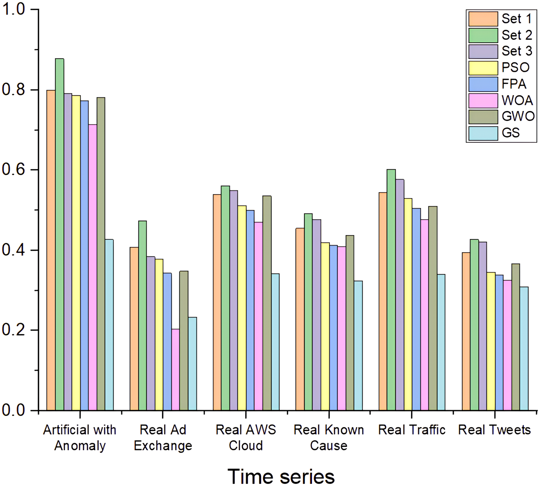
The results presented in Fig. 9 highlight the comparison of the proposed method, using hyperparameters (Sets 1, Set 2, and Set 3) against five optimization algorithms: PSO, FPA, WOA, GWO, and GS. The HABCOeSNN, when utilizing Set 2 hyperparameters, consistently outperforms the other configurations, achieving the highest F1-scores in most time series, such as ArtificialWithAnomaly for (0.878) and RealTraffic with (0.603). This indicates that the hyperparameters in Set 2 significantly enhance the generalization ability of the suggested method, allowing for more accurate anomaly detection in both synthetic and real-world data. Although algorithms like PSO and FPA yield competitive results, they generally underperform compared to the proposed method, particularly in complex datasets such as RealAdExchange and RealTweets.
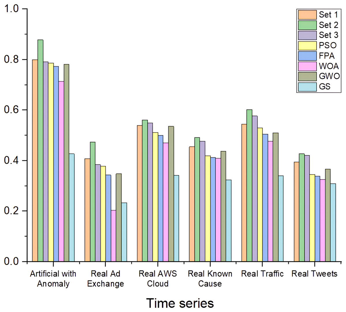
Figure 9: F1-score of HABCOeSNN against PSO, GWO, FPA, WOA, and GS algorithms on the NAB dataset.
Significance analysis
To ascertain the efficacy of the HABCOeSNN, a one-way analysis of variance (ANOVA) test was conducted to determine whether a statistically significant difference exists between the HABCOeSNN and other state-of-the-art methods. The high F-statistic and a corresponding p-value of less than 0.05 imply that the performance differences are statistically significant (Barbara & Fidell, 2013). As illustrated in Table 16, the HABCOeSNN utilizing Set 2 hyperparameters demonstrated a pronounced superiority over a range of benchmark anomaly detectors, as evidenced by high F-statistic values and extremely low p-values (p < 0.05). These findings support the resilience of the HABCOeSNN and reliability with Set 2 hyperparameters, establishing it as a novel and effective solution for unsupervised anomaly detection in streaming data.
| Approaches | P-value | HABCOeSNN |
|---|---|---|
| Bayesian changepoint | 0.000007 | Significant |
| Context OSE | 0.000007 | Significant |
| EXPoSE | 0.000007 | Significant |
| HTM JAVA | 0.000009 | Significant |
| KNN CAD | 0.000007 | Significant |
| Numenta | 0.000009 | Significant |
| NumentaTM | 0.000009 | Significant |
| Relative Entropy | 0.000008 | Significant |
| Skyline | 0.000013 | Significant |
| Twitter ADVec | 0.000008 | Significant |
| Windowed Gaussian | 0.000010 | Significant |
| DeepAnT | 0.000136 | Significant |
| OeSNN-UAD | 0.006593 | Significant |
Ablation study
To determine the contribution of the components in HABCOeSNN, an ablation study is presented across both the Yahoo Webscope and NAB datasets. Three configurations are assessed in the ablation study: (1) standard OeSNN with default hyperparameters and no optimization, (2) Offline-Optimized OeSNN, in which hyperparameters are adjusted once using ABC on a validation subset and then fixed, and (3) the full HABCOeSNN model with adaptive ABC optimization in real-time. As reported in Table 17, standard OeSNN achieved an average F1-score of 0.376 across six NAB time series categories, which improved to 0.436 with Offline-Optimized OeSNN. The HABCOeSNN model significantly outperformed both, reaching an average F1-score of 0.572. Similarly, in the Yahoo Webscope benchmark, the average F1-score increased from 0.646 (Standard OeSNN) to 0.824 (Offline-Optimized OeSNN), with the proposed HABCOeSNN further improving performance to 0.848.
| Data sets | Categories | Standard OeSNN |
Offline-optimized OeSNN | HABCOeSNN |
|---|---|---|---|---|
| NAB | Artificial with Anomaly | 0.568 | 0.591 | 0.878 |
| Real Ad Exchange | 0.270 | 0.351 | 0.473 | |
| Real AWS Cloud | 0.290 | 0.385 | 0.561 | |
| Real Known Cause | 0.339 | 0.401 | 0.491 | |
| Real Traffic | 0.501 | 0.557 | 0.603 | |
| Real Tweets | 0.288 | 0.331 | 0.427 | |
| Yahoo Webscope |
A1Benchmark | 0.716 | 0.742 | 0.852 |
| A2Benchmark | 0.737 | 0.838 | 0.942 | |
| A3Benchmark | 0.694 | 0.918 | 0.847 | |
| A4Benchmark | 0.438 | 0.798 | 0.749 |
These results reveal a clear and consistent performance gain at each step of model enhancement. The notable improvements from static ABC optimization validate that proper hyperparameter tuning is critical to effective anomaly detection using evolving spiking neural networks. However, the additional boost achieved by HABCOeSNN underscores the importance of online, adaptive optimization in non-stationary streaming contexts. Overall, the ablation results validate that both optimization and adaptivity are essential, and their combination in HABCOeSNN is key to achieving robust, real-time anomaly detection in unsupervised streaming environments.
Conclusions
This study introduced a hybrid Artificial Bee Colony (ABC) algorithm with an Online Evolving Spiking Neural Network (OeSNN), termed HABCOeSNN, for unsupervised anomaly detection in streaming data. The ABC was employed to explore the hyperparameter space and identify the optimal configurations, thereby overcoming the challenge of manually tuning the hyperparameters of the OeSNN. Three sets of hyperparameters were investigated: Set 1 (window size (Wsize) and anomaly classification factor (ε)); Set 2 (similarity value (SIM), modulation factor (MOD), and threshold factor (C)); and Set 3 (combination of all five parameters).
To ensure robust evaluation, the HABCOeSNN was assessed on two benchmark datasets, Yahoo Webscope and Numenta Anomaly Benchmark (NAB), using several assessment criteria. Furthermore, the study employed Multi-Criteria Decision-Making (MCDM) to produce performance validation beyond single-metric evaluation, to ensure enhanced accuracy in anomaly detection. Moreover, HABCOeSNN performance was compared against five state-of-the-art optimization techniques: PSO, FPA, GWO, WOA, and Grid Search, along with other well-known classifiers, Random Forest, SVM, and kNN. Additionally, an ablation study was conducted to determine the contribution of each component in HABCOeSNN.
The result demonstrated consistent improvements in detection performance with HABCOeSNN achieving significantly higher F1-scores across both datasets, as confirmed by statistical validation using one-way ANOVA. These findings emphasize the crucial importance of precise hyperparameter optimization in enhancing the learning capabilities of the OeSNN, particularly with respect to the hyperparameters SIM, MOD, and C, which were identified as the most effective configurations for anomaly detection problems.
The proposed method can be further enhanced in the future by simultaneously refining the OeSNN architecture and hyperparameters, utilizing a multi-objective optimization approach to effectively balance accuracy and computational complexity. Following the “No Free Lunch” theorem, more effort might be focused on hybridized HABCOeSNN with different metaheuristic algorithms to benefit from the advantages of various optimization techniques to improve anomaly detection accuracy. The computational cost will also be investigated further to create a fair comparison with alternative approaches. Finally, extending the assessment to include real-world, high-volume streaming data scenarios would provide deeper insights into its practical deployment potential.